Circular Horn Antenna - CST2013 MWS Examples

下载CST设计文件

General Description

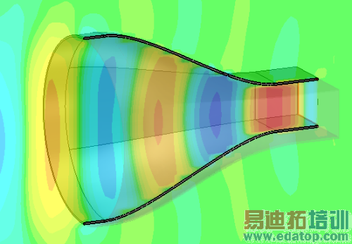
This example shows the calculation of farfields and electric fields of a horn antenna. The antenna consists of a rectangular waveguide, which is connected with a circular horn by the loft feature. Also the setup of result templates is shown, which are stored during parameter sweeping and optimization runs.

Structure Generation

The antenna is created using a basic brick and cylinder. More advanced operations are the usage of the local working coordinate system before defining the cylinder and especially the loft operation to connect rectangular and circular faces. At the end (after boolean adding the 3 individual objects), the Shell-feature is applied to create a finite wall thickness.

Solver Setup

A waveguide port is defined on the open side of the rectangular waveguide to stimulate the antenna. All calculation domain boundary conditions are set to "open". Magnetic and electric symmetry planes are used to reduce the calculation time. Besides standard e-field and farfield monitors also a Result Template is setup to store and compare the farfield gain during mesh adaption runs, parameter sweeping or optimization runs.

Post Processing

The electric field distribution can be accessed in the navigation tree in the subfolders of 2D/3D Results E-Field. The farfield patterns are listed in subfolders of Farfields in the navigation tree. For the farfield, the phase center calculation has been activated. The phase center is determined for the phi component within the xz plane, i.e. the H plane in an angular width of 15 degree around the main lobe direction. To cross check the phase center position, it is entered as origin in the farfield plot dialog. Switching the coordinate system to Ludwig 3 in the axis tab, changing to E field in the plot mode tab of the farfield plot dialog and selecting the Ludwig 3 Vertical Phase component in the navigation tree, one can see the constant phase around the main lobe.

In addition, the temporal development of the electric phi and magnetic theta component recorded by the farfield probes can be studied in the 1D Results Probes E-Farfield and 1D Results Probes H-Farfield folders of the navigation tree.