Rectangular Waveguide Tutorial - CST2013 MWS Examples

Contents

Geometric Construction and Solver Settings. 2

Introduction and Model Dimensions. 2

Geometric Construction Steps. 3

Calculation of Fields and S-Parameters. 12

Transient Solver 12

Transient Solver Results. 13

Accuracy Considerations. 17

Frequency Domain Solver 20

Frequency Domain Solver Results. 22

Accuracy Considerations. 25

Getting More Information. 26

Geometric Construction and Solver Settings

Introduction and Model Dimensions

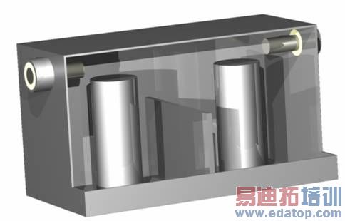
In this tutorial you will learn how to simulate rectangular waveguide devices. As a typical example for a rectangular waveguide, you will analyze a well-known and commonly used high frequency device: the Magic Tee. The acquired knowledge of how to model and analyze this device can also be applied to other devices containing rectangular waveguides.

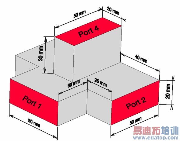
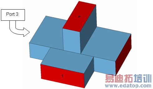
The main idea behind the Magic Tee is to combine an E-plane and an H-plane T-junction waveguide (see the figure below for an illustration and the dimensions). Although CST MICROWAVE STUDIO can provide a wide variety of results, this tutorial concentrates solely on the S-parameters and electric fields. In this particular case, port 1 and port 4 are de-coupled, so one can expect S14 and S41 to be very small.

We strongly suggest that you carefully read through the CST STUDIO SUITE - Getting Started and CST MICROWAVE STUDIO - Workflow and Solver Overview manual before starting this tutorial.

Geometric Construction Steps

After you have started CST STUDIO SUITE you have the possibility to create a new project template, that will pre-define basic settings for the simulation of your specific application. In this tutorial the settings are optimized for an RF waveguide component, consequently the units are set to mm and GHz.

Because the background material (that will automatically enclose the model) is specified as being a perfect electrical conductor, you only need to model the air-filled parts of the waveguide device. In the case of the Magic Tee, a combination of three bricks is sufficient to describe the entire device. In addition, all boundaries are set to be perfect electrical conductors, which is also already defined as default.

o Create a New Project

After launching the CST STUDIO SUITE you will enter the start screen showing you a list of recently opened projects and allowing you to specify the application which suits your requirements best. The easiest way to get started is to configure a project template which defines the basic settings that are meaningful for your typical application. Therefore click on the Create Project button in the New Project section.

Next you should choose the application area, which is Microwaves & RF for the example in this tutorial and then select the workflow by double-clicking on the corresponding entry.

For the Rectangular Waveguide device, please select Circuits & Components Waveguide Couplers & Dividers Time Domain Solver .

At last you are requested to select the units which fit your application best. For the Rectangular Waveguide device, please select the dimensions as follows:

For the specific application in this tutorial the other settings can be left unchanged. After clicking the Next button, you can give the project template a name and review a summary of your initial settings:

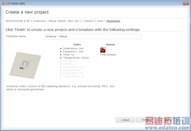
Finally click the Finish button to save the project template and to create a new project with appropriate settings. CST MICROWAVE STUDIO will be launched automatically due to the choice of the application area Microwaves & RF.

Please note: When you click again on the File: New and Recent you will see that the recently defined template appears below the Project Templates section. For further projects in the same application area you can simply click on this template entry to launch CST MICROWAVE STUDIO with useful basic settings. It is not necessary to define a new template each time. You are now able to start the software with reasonable initial settings quickly with just one click on the corresponding template.

Please note: All settings made for a project template can be modified later on during the construction of your model. For example, the units can be modified in the units dialog box (Home:Settings Units ) and the solver type can be selected in the Home:Simulation Start Simulation drop-down list.

o Define Working Plane Properties

Usually, the next step is to set the working plane properties in order to make the drawing plane large enough for your device. Because the structure has a maximum extension of 100 mm along a coordinate direction, the working plane size should be set to at least 100 mm. The raster width and snap width are set to 10 and 5 respectively. These settings can be changed in a dialog box that opens after selecting View: Working Plane Working Plane Properties.

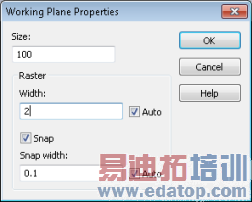
Change the settings in the working plane properties window to the values given above before pressing the OK button.

o Define the First Brick

Now you can create the first brick:

This is most easily accomplished by selecting Modeling: Shapes Brick .

CST MICROWAVE STUDIO now asks you for the first point of the brick. The current coordinates of the mouse pointer are shown in the bottom right corner of the drawing window in an information box. After you double-click on the point x=50 and y=10, the information box will show the current mouse pointers coordinates and the distance (DX and DY) to the previously picked position. Drag the rectangle to the size DX=-100 and DY=-20 before double-clicking to fix the dimensions. CST MICROWAVE STUDIO now switches to the height mode. Drag the height to h=50 and double-click to finish the construction. You should now see both the brick, shown as a transparent model, and a dialog box, where your input parameters are shown. If you have made a mistake during the mouse based input phase, you can correct it by editing the numerical values. Create the brick with the default component and material settings by pressing the OK button:

The new solid now should look as follows:

You have just created the waveguide connecting ports 2 and 3. Adding the waveguide connection to port 1 will introduce another of CST MICROWAVE STUDIO′s features, the Working Coordinate System (WCS). It allows you to avoid making calculations during the construction period. Lets continue and discover this tools advantages.

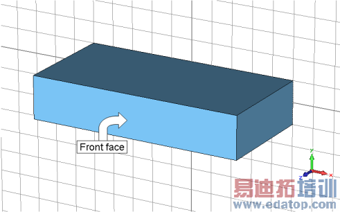
o Align the WCS with the Front Face of the First Brick

To add the waveguide belonging to port 1 to the front face, as shown in the above picture, please select Modeling: WCS Align WCS or just use shortcut W. Now simply double-click on the front face of the brick. This action moves and rotates the WCS so that the working plane (uv plane) coincides with the selected face.

o Define the Second Brick

With the WCS in the right location, creating the second brick is quite simple. Start again the brick creation mode by selecting Modeling: Shapes Brick . Please remember that all values used for shape construction are relative to the uvw coordinate system as long as the WCS is active.

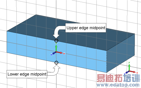
The new brick should be aligned with the edge midpoints of the first brick as shown in the picture above. Without leaving the current brick creation mode, you should pick the lower edges midpoint by simply activating the appropriate pick tool Modeling: Picks Pick Point Pick Edge Center or use the shortcut M). Now all edges become highlighted and you can simply double-click on the first bricks lower edge as shown in the picture. Then, continue with the brick creation by repeating the procedure for the bricks upper edge.

Because you have now selected two points that are located on a line, you will be requested to enter the width of the brick. Please note that this step will be skipped if the two previously picked points already form a rectangle (not only a line). Now you should drag the width of the brick to w=50 (watch the coordinate display in the lower right corner of the drawing window) and double-click on this location.

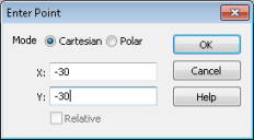
Finally, you must specify the bricks height. Therefore, drag the mouse to the proper height (h=30) and double-click on this location. Please note that instead of specifying coordinates with the mouse (as we have done here), you can also press the TAB key whenever a coordinate is requested. This will open a dialog box where you can specify the coordinates numerically.

After the bricks interactive construction is completed, a dialog box will again appear showing a summary of the bricks parameters.

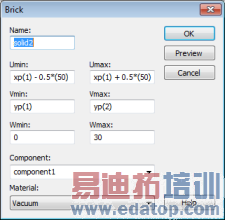
Some of the coordinate fields now contain mathematical expressions because some of the points were entered using the pick tools. Here, the functions xp(1), yp(1) represent the point coordinates of the first picked point (the midpoint of the first bricks lower edge). Analogously, the functions xp(2) and yp(2) correspond to the upper edges midpoint.

Because you are currently constructing the inner waveguide volume, you can still keep the default Vacuum Material setting and the same Component (component1) as for the first brick.

Please note: The use of different components allows you to gather several solids into specific groups, independent of their material behavior. For this tutorial, however, it is convenient to construct the complete structure as a single component.

Finally, you should confirm the bricks creation again by pressing the OK button. Let's now construct the third brick.

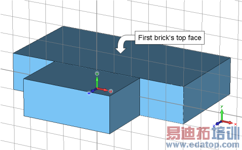
o Align the WCS with the First Bricks Top Face

The next brick should be aligned with the top face of the first brick. To align the local coordinate system with this face, please select Modeling: WCS Align WCS or use shortcut W and then directly double-click on the desired face.

o Construct the Third Brick

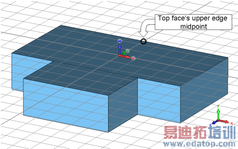
Please enter again the brick creation mode by selecting Modeling: Shapes Brick . When you are requested to enter the first point, you should activate the center edge pick tool (shortcut M), as you did for the previous brick, and double-click on the top faces upper edge midpoint (see picture above).

The next step is to drag the mouse in order to specify the extension of DV=-50 along the v direction (hold down the Shift key while dragging the mouse to restrict the coordinate movement to the v direction only) and double-click on this location. Afterwards, you should specify the width of the brick as w=20 and the height as h=30 in the same manner, or by entering these values numerically using the Tab key.

The last brick is also created as a vacuum material and belongs to the component component1. Finally, confirm these settings in the brick creation dialog box. Now the structure should look as follows:

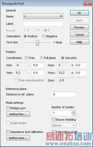
o Define Port 1

In the next step you will assign the first port to the front face of the Magic Tee (see picture above). The easiest way to do this is to pick the port face by selecting Modeling: Picks Picks Pick Points, Edges or Faces or using shortcut S and then double-click on the desired face.

Once the ports face is selected you can open the waveguide port dialog box either by selecting Simulation: Sources and Loads Waveguide Port . The settings in the waveguide port dialog box will automatically specify the extension and location of the port according to the bounding box of any previously picked elements (faces, edges or points).

In this case, you can simply accept the default settings and press OK to create the port. The next step is the definition of ports 2, 3 and 4.

o Define Ports 2, 3, 4

Repeat the last steps (pick face and create port) to define port 2, port 3 and port 4. After you have completed this step, your model should look like the below figure. Please double-check your input before proceeding to the solver settings.

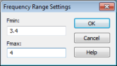
o Define the Frequency Range

The frequency range for this example extends from 3.4 GHz to 4 GHz. Change Fmin and Fmax to the desired values in the frequency range settings dialog box by selecting Simulation: Settings Frequency . Please note that the currently selected units are shown in the status bar.

o Define Field Monitors

Because the amount of data generated by a broadband time domain calculation is huge even for relatively small examples, it is necessary to define which field data should be stored before the simulation is started. CST MICROWAVE STUDIO uses the concept of monitors in order to specify which types of field data to store. In addition to the type, you also must specify whether the field should be recorded at a fixed frequency or at a sequence of time samples. You can define as many monitors as necessary to get different field types or fields at various frequencies. Please note that an excessive number of field monitors may significantly increase the memory space required for the simulation.

To add a field monitor, please select Simulation: Monitors Field Monitor :

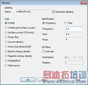
In this example, you should define an electric field monitor (Type = E-Field) at the center Frequency of 3.6 GHz before pressing the OK button to store the settings. The green box indicates the volume in which the fields will be recorded.

Calculation of Fields and S-Parameters

A key feature of CST MICROWAVE STUDIO is the Method on Demand approach that allows a simulator or mesh type that is best suited for a particular problem. Another benefit is the ability to compare the results obtained by completely independent approaches. We demonstrate this strength in the following sections by calculating fields and S-parameters with the transient solver and the frequency domain solver. In this case, the transient simulation uses a hexahedral mesh while the frequency domain calculation is performed with a tetrahedral mesh. Both sections are self-contained and it is sufficient to work through only one of them, depending on which solver you are interested in. The section on the frequency domain solver also provides a comparison with the transient simulation.

Transient Solver

o Transient Solver Settings

The transient solver parameters are specified in the solver control dialog box that can be opened by selecting Simulation: Solver Start Simulation Time Domain Solver or directly from within your Home Ribbon Home: Simulation Start Simulation :

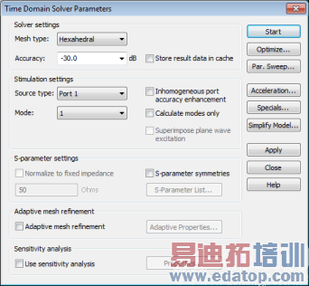
You should now specify whether the full S-matrix should be calculated or if a subset of this matrix is sufficient. For the Magic Tee device we are interested in the input reflection at port 1 and in the transmission from port 1 to the other three ports (2, 3 and 4).

Accordingly, we only need to calculate the S-parameters S1,1, S2,1, S3,1 and S4,1. All of the S-parameters can be derived by an excitation at port 1. Therefore, you should change the Source type field in the Stimulation settings frame to Port 1. If you leave this setting at All Ports, the full S-matrix will be calculated.

Finally, press the Start button to begin the calculation. A progress indicator appears in the Progress window displaying some information about the calculation. If any error or warning messages are produced by the solver, they will be displayed in the Messages window.

Transient Solver Results

Congratulations, you have simulated the Magic Tee! Lets review the results.

o 1D Results (Port Signals, S-Parameters)

First, we observe the port signals by opening the 1D Result folder in the navigation tree and clicking on the Port signals folder:

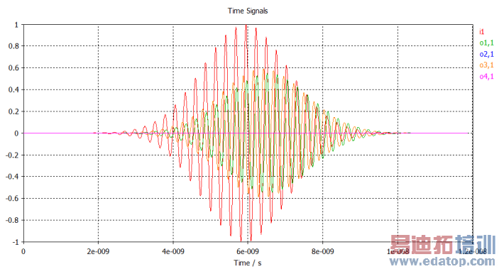
This plot shows the incident and reflected or transmitted wave amplitudes at the ports versus time. The incident wave amplitude is called i1, the reflected wave amplitude is o1,1 and the transmitted wave amplitudes are o2,1, o3,1 and o4,1. You can see that the transmitted wave amplitudes o2,1 and o3,1 are delayed and distorted (note that o2,1 and o3,1 are identical, so do not be concerned if you only see one curve).

The S-parameters can be plotted by clicking on the 1D Results S-Parameters folder and selecting 1D Plot: Plot Type dB for dB representation:

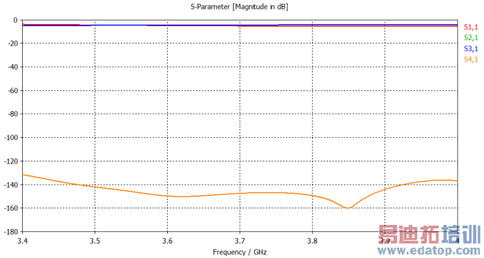
As expected, the transmission to port 4 (S4,1) is extremely small (-150 dB is close to the solvers noise floor). It is obvious that this simple device is very poorly matched so that the transmission to ports 2 and 3 is of the same order of magnitude as the input reflection at port 1.

o 2D and 3D Results (Port Modes and Field Monitors)

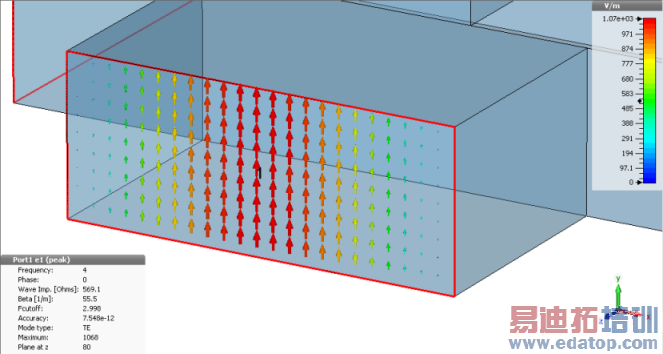
Finally, we will review the 2D and 3D field results. We will first inspect the port modes that can be easily displayed by opening the 2D/3D Results Port Modes Port1 folder from the navigation tree. To visualize the electric field of the fundamental port mode you should click on the e1 subfolder.

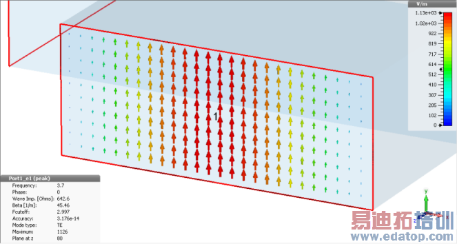
Because we have selected the main entry, a 3D vector plot is shown. Selecting either of the subentries will produce a scalar plot. The plot also shows some important properties of the mode such as mode type, cut-off frequency and propagation constant. The port modes at the other ports can be visualized in the same manner.

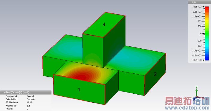
The full three-dimensional electric field distribution in the Magic Tee can be shown by selecting the 2D/3D Results E-Field efield (f=3.6)[1] folder from the navigation tree. If the Normal item is clicked, the field plot will show a three dimensional contour plot of the electric field normal to the surface of the structure.

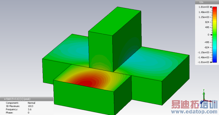
You can display an animation of the fields by checking the Animate Fields option in the context menu (right mouse click in the plot window). The appearance of the plot can be changed in the plot properties dialog box, that can be opened by selecting 2D/3D Plot: Plot Properties Properties or Plot Properties from the context menu. Alternatively, you can double-click on the plot to open this dialog box.

Accuracy Considerations

In this case, the transient S-parameter calculation is mainly affected by two sources of numerical inaccuracies:

1. Numerical truncation errors introduced by the finite simulation time interval.

2. Inaccuracies arising from the finite mesh resolution.

In the following section we provide hints on how to minimize these errors and obtain highly accurate results.

o Numerical Truncation Errors Due to Finite Simulation Time Intervals

As a primary result, the transient solver calculates the time varying field distribution that results from an excitation with a Gaussian pulse at the input port. Thus, the signals at the ports are the fundamental results from which the S-parameters are derived using a Fourier Transform.

Even if the accuracy of the time signals themselves is extremely high, numerical inaccuracies can be introduced by the Fourier Transform that assumes the time signals have completely decayed to zero at the end. If the latter is not the case, a ripple is introduced into the S-parameters that affects the accuracy of the results. The amplitude of the excitation signal at the end of the simulation time interval is called truncation error. The amplitude of the ripple increases with the truncation error.

Please note that this ripple does not move the location of minima or maxima in the S-parameter curves. Therefore, if you are only interested in the location of a peak, a larger truncation error is tolerable.

The level of the truncation error can be controlled using the Accuracy setting in the transient solver control dialog box. The default value of -30 dB (moderate) will usually give sufficiently accurate results for coupler devices. However, to obtain highly accurate results for waveguide structures it is sometimes necessary to increase the accuracy to -40 dB (high) or- 50 dB (very high).

If you find large ripples in the S-Parameter, it might be necessary to further increase the solvers accuracy setting or use the AR-Filter feature that is explained in more detail in the online help.

o Effect of the Mesh Resolution on the S-parameters Accuracy

The inaccuracies arising from the finite mesh resolution are usually more difficult to estimate. The only way to ensure the accuracy of the solution is to increase the mesh resolution and recalculate the S-parameters. If these results no longer significantly change when the mesh density is increased, then convergence has been achieved.

In the example above, you have used the default mesh that has been automatically generated by an expert system. The easiest way to prove the accuracy of the results is to use the fully automatic mesh adaptation that can be switched on by checking the Adaptive mesh refinement option in the solver control dialog box:

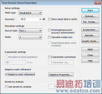
After activating the adaptive mesh refinement tool, you should now start the solver again by pressing the Start button. After a couple of minutes (during which the solver is running through mesh adaptation passes), the following dialog box will appear:

This dialog box informs you that the desired accuracy limit (2% by default) could be met by the adaptive mesh refinement. Because the expert systems settings have now been adjusted such that this accuracy is achieved, you may switch off the adaptation procedure for subsequent calculations (e.g. parameter sweeps or optimizations).

You should now confirm the deactivation of the mesh adaptation by pressing the Yes button.

After the mesh adaptation procedure is complete, you can visualize the maximum difference of the S-parameters for two subsequent passes by selecting 1D Results Adaptive Meshing Delta S from the navigation tree:

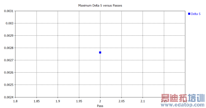
As you can see, the maximum deviation of the S-parameters is below 0.5%, indicating that the expert system based meshing would have been fine for this example even without running the mesh adaptation procedure.

The convergence process of the input reflection S1,1 during the mesh adaptation can be visualized by selecting 1D Results Adaptive Meshing S-Parameters S1,1 from the navigation tree and selecting 1D Plot: Plot Type dB to show the results in dB representation :

The convergence process of the other S-parameters can be visualized in the same manner. Please note that S4,1 is extremely small (< -120dB) in this example; its variations are mainly due to the numerical noise and are therefore ignored by the automatic mesh adaptation procedure.

The advantage of this expert system based mesh refinement procedure over traditional adaptive schemes is that the mesh adaptation needs to be carried out only once for each device to determine the optimum settings for the expert system. There is subsequently no need for time consuming mesh adaptation cycles during parameter sweeps or optimizations.

Please note: Refer to the CST MICROWAVE STUDIO - Workflow and Solver Overview manual how to use Template Based Postprocessing for automated extraction and visualization of arbitrary results from various simulation runs.

Frequency Domain Solver

CST MICROWAVE STUDIO offers a variety of frequency domain solvers specialized for different types of problems. They differ not only by their algorithms but also by the grid type they are based on. The general purpose frequency domain solver is available for hexahedral grids, as well as for tetrahedral grids. In this tutorial we will use a tetrahedral mesh. The availability of a frequency domain solver within the same environment offers a very convenient means of cross-checking results produced by the time domain solver.

o Making a Copy of Transient Solver Results

Before performing a simulation with the frequency domain solver, you may want to keep the results of the transient solver in order to compare the two simulations. The copy of the current results is obtained as follows: Select, for example, the S-Parameters folder in 1D Results, then press Ctrl+c and Ctrl+v. The copies of the results will be created in the selected folder. The names of the copies will be S1,1_1, S2,1_1 etc. You may rename them to S1,1_TD, S2,1_TD and so on with the Rename command from the context menu. Use Add new tree folder from the context menu to create an extra folder. Please note that at the current time it is not possible to make a copy of 2D or 3D results.

o Frequency Domain Solver Settings

In order to now start a frequency domain simulation the currently active solver has to be changed to Home: Simulation Start Simulation Frequency Domain Solver :

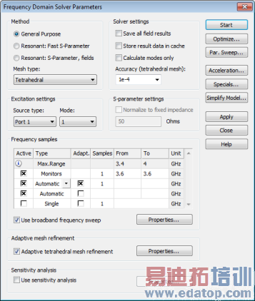
There are three different methods to choose from. For the example here, please choose the General Purpose frequency domain solver. In the Mesh Type combo box you may choose Hexahedral or Tetrahedral Mesh. Please choose Tetrahedral Mesh.

You should now specify whether the full S-matrix should be calculated or if a subset of this matrix is sufficient. For the Magic Tee device we are interested in the input reflection at port 1 and in the transmission from port 1 to the other three ports (2, 3 and 4).

Consequently, we only need to calculate the S-parameters S1,1, S2,1, S3,1 and S4,1. All of the S-parameters can be derived by an excitation at port 1. Therefore, you should change the Source type field in the Excitation settings frame to Port 1 unless already done. If this is set to All Ports, the full S-matrix will be calculated.

S-parameters in the frequency domain are obtained by solving the field problem at different frequency samples. These single S-parameter values are then used by the broadband frequency sweep to get the continuous S-parameter values. With the default settings in the frequency samples frame the number and the position of the frequency samples are chosen automatically in order to meet the required accuracy limit throughout the entire frequency band.

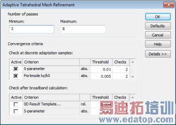
Unlike the time domain solver, the tetrahedral frequency domain solver should always be used with the Adaptive tetrahedral mesh refinement. Otherwise, the initial mesh may lead to a poor accuracy. Therefore, the corresponding check box is activated by default. All other settings may be left unchanged.

After everything is ready, you may press Start to begin the calculation.

Because the old results will be overwritten when starting a different solver, the following warning message appears:

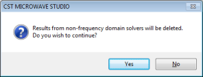
Press Yes to acknowledge the deletion. A progress bar will appear at the bottom of the main frame as soon as the solver starts. Additional information about the simulation progress will be shown in the message window that will be activated automatically, if necessary.

Frequency Domain Solver Results

After the desired accuracy for the S-parameter has been reached the simulation stops.

o 1D Results (S-Parameters)

As for the transient solver run, you can view the S-parameters by selecting 1D Results S-Parameters in the navigation tree and selecting 1D Plot: Plot Type dB for dB representation.

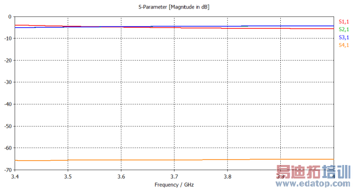
Similar to the case of transient solver, an extremely small transmission to port 4 (S4,1) is observed here. In addition, you can conclude that the other S-parameters have at least the same order of magnitude as the S-parameters computed with the transient solver.

The next figure shows the S-parameters S1,1 and S1,2 for both transient and frequency domain solvers plotted in the same graph. This can be done by copying all these results to an extra folder.

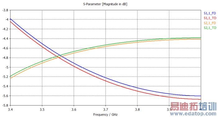
As you can see, the results agree very well. For this specific structure, the transient solver does provide more accurate results by default. The accuracy of the frequency domain simulation can be increased by lowering the accuracy limit for the adaptive mesh refinement.

o 2D and 3D Results (Port Modes and Field Monitors)

The 2D and 3D field results can be found in the 2D/3D Results folder of the navigation tree. The electric field of the fundamental mode at port 1 can be visualized by selecting the Port Modes Port1 e1 folder:

The mode properties shown in the lower left corner of the field plot are close to those computed with the transient solver. Note that the frequency of the mode is not exactly equal to the frequency used by the transient solver. For inhomogeneous ports the frequency domain solver calculates the modes for every frequency sample, in this example the ports are calculated only once, here at a frequency of 4GHz.

The three-dimensional electric field distribution in the Magic Tee can be visualized by opening the 2D/3D Results E-Field efield (f=3.6)[1] folder of the navigation tree. After selecting the Normal item the field plot will show a three dimensional contour plot of the electric field normal to the surface of the structure.

You can display an animation of the fields by checking the Animate Fields option in the context menu (right mouse click in the plot window). The appearance of the plot can be changed in the plot properties dialog box, that can be opened by selecting 2D/3D Plot: Plot Properties Properties or Plot Properties from the context menu. Alternatively, you can double-click on the plot to open this dialog box.

The next section describes how to influence the mesh refinement and improve the quality of the computed field distribution.

Accuracy Considerations

The results of the frequency domain solver using the tetrahedral mesh are mainly affected by the inaccuracies arising from the finite mesh resolution. In the case of a tetrahedral mesh the adaptive mesh refinement is switched on by default. The mesh adaptation is performed by checking the convergence of the S-parameter values at the highest simulation frequency. The adaptation is oriented towards achieving highly accurate S-parameter calculations.

In the presented example three mesh adaptation passes have been performed according to the Minimum number setting in the Number of passes frame. This setting can be accessed by pressing Properties in the Adaptive mesh refinement frame of the Frequency Domain Solver Parameters dialog:

Getting More Information

Congratulations! You have just completed the Rectangular Waveguide tutorial that should have provided you with a good working knowledge on how to use transient and frequency domain solvers to calculate S-parameters. The following topics have been covered:

1. General modeling considerations, using templates, etc.

2. Use picked points to define objects relatively to each other.

3. Define ports.

4. Define frequency ranges.

5. Define field monitors.

6. Start the transient or the frequency domain solver.

7. Visualize port signals and S-parameters.

8. Visualize port modes and field monitors.

9. Check the truncation error of the time signals.

10. Obtain accurate and converged results using the automatic mesh adaptation.

You can obtain more information for each particular step from the online help system that can be activated either by pressing the Help button in each dialog box or by pressing the F1 key at any time to obtain context sensitive information.

In addition to this tutorial, you can find some more S-parameter calculation examples in the examples folder in your installation directory. Each of these examples contains a Readme item in the navigation tree that will give you some more information about the particular device.

Finally, you should refer to the Online documentation for more in-depth information on issues such as the fundamental principles of the simulation method, mesh generation, usage of macros to automate common tasks, etc.