Inhomogeneously Biased Circulator - CST2013 MWS Examples

General Description

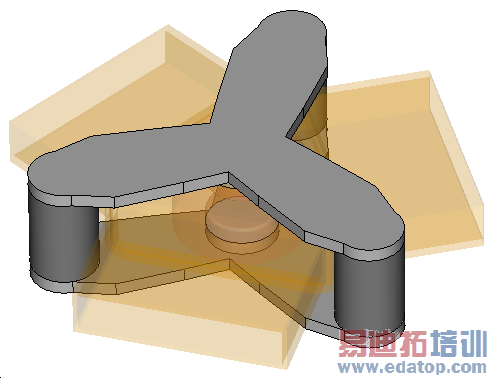
In this example the characteristic behavior of an inhomogeneously biased H-plane three port circulator is presented by the calculation of the corresponding S-parameters with the tetrahedral frequency domain solver.

The main part of the structure is the field rotation domain, containing two ferrite disks embedded in a teflon cylinder. Three rectangular waveguides are responsible for the in and out coupling of the fundamental TE mode. In case that the ferrite material is biased by a static magnetic field, the circulator shows a non-reciprocal behavior, which is typical for microwave devices using gyrotropic media.

Before the frequency domain simulation actually starts, a nonlinear static magnetic field simulation is performed to obtain the biasing field for the ferrite material. The final material properties of the ferrite material are then calculated according to this field.

The calculated field distributions are visualized by help of 3D field monitors, in particular the powerflow and current density. The static magnetic field and magnetic flux distributions are also available.

The entire results of the static simulation can be found by opening the project "StatFerr.cst" stored in the "inhombiasedcircResultCpldProj" folder, where "inhombiasedcirc" is the name of the project.

A very similar structure has also been simulated with a constant biasing field using the Time Domain and the Frequency Domain General Purpose Tetrahedral solver.

Structure Generation

The main part of the circulator is constructed with the definition of a curve and its extrude functionality, while all other elements are modelled as solid shapes, applying mirror and shell and rotation transformations. Using the local coordinate system offers the possibility to create the different parts relative to each other.

For the magnetostatic simulation a relatively large surrounding space block is created to ensure sufficient distance to the boundaries. The material model for this block is different for low frequency and high frequency problem types: the material properties of "Vacuum Outer" are equal to vacuum for the "default" problem type which is used by the magnetostatic simulation since no low frequency material properties have been defined otherwise. For the high frequency simulation this block is treated as PEC, as can be seen if the problem type is switched to "High Frequency" in the material properties of "Vacuum Outer." This solid block of PEC does not have any effect in the high frequency simulation since perfectly conducting materials have zero fields.

The anisotropic and dispersive material character of the biased ferrite as well as the nonlinearity of the magnet components are defined by the corresponding material parameters.

Solver Setup

Three non orthogonal waveguide ports are defined at the ends of the given waveguides to perform the S-parameter calculation in the frequency range from 13 to 17 GHz. For the static simulation permanent magnets properties are assigned to the three cylinders.

The tetrahedral frequency domain solver is started with 3D mesh adaption and the Calculate static H-Field for Ferrites option switched on.

In order to get an additional visualization of the non-reciprocal wave propagation several 3D field monitors (electric and magnetic field, powerflow) are defined at the operation frequency of 15 GHz.

Post Processing

The resulting scattering parameters of the frequency domain calculation are listed in the navigation tree in the folder 1D Results. Here you can also find information about the performed mesh adaption and the solver convergence.

Regarding the absolute value of the S-parameters the asymmetric coupling of the field energy from port No.1 to port No.2 is obvious. This result can be visualized more impressively by plotting the monitored 3D fields, which can be found in the folder 2D/3D Results.

To easily check the applied static magnetic field strength the mean value of the z-component of the recorded H-Field is calculated along a previously defined wire inside the ferrite. This operation is done by using the "Template based postprocessing" feature. The mean value can be found in the result tree in: Tables 0D Results curve1_H_Mean.