CST2013: General 1D / Fourier Transform

Result TemplatesTemplate Based Post Processing

This template allows to calculate the Fourier Transform of a given function, as well as its inverse. Additional options are (inverse) Fourier Series and Power Spectrum Density (PSD).

Fourier Transform (FT)

This will calculate the FT of a given function, specified in the '1D Results' box. In almost all cases, the input function will be real-valued. However, complex-valued input functions are allowed for completeness. The FT will be calculated in the frequency interval between Fmin and Fmax, as specified by the user. Mathematically, the FT returns positive and negative frequencies. For real-valued functions, the positive and negative side of the FT are the complex conjugate of each other and it is common to plot only the positive frequencies. If this is desired, Fmin should be larger than or equal to zero, and the checkbox 'To half-sided spectrum' should be checked.

The number of samples of the input function and the resulting FT are critical for accurate and physically meaningful results. Due to the Nyquist-Shannon sampling theorem, the input function should be sampled with at least twice the specified Fmax. Violating this requirement will usually result in aliasing effects. The user may tick the checkbox 'Resample with Nyquist rate before evaluation' to resample the input function with an equidistant time step of 1/(2*Fmax) before calculating the FT. Although the algorithm is able to handle functions with non-equidistant sampling, it is recommended to resample such functions equidistantly, also by activating the checkbox 'Resample with Nyquist rate before evaluation'.

The number of samples for the FT can be specified in the textbox labeled as '# of samples'. The higher this number, the better the resolution in the frequency domain will be. The 'Auto' setting will choose the number of samples such that a frequency of 1/(2*(t1-t0)) can be resolved, where t1 and t0 are the highest and the lowest x-value of the input function.

The user also has the option of changing the default normalization of the FT. The default setting of "1" in FT and inverse FT (IFT) ensures that IFT(FT(f)) = f. (Internally, this means that the FT will be normalized with "1" and the IFT will be normalized with "1/2*Pi".) If the user decides to change the normalization to "alpha" for the FT, the normalization for the IFT should be set to "1/alpha" to ensure that IFT(FT(f)) = f.

Please note that the Fourier Transform does not assume the input to be periodic. If the input function is given between t0 and t1, all input values before t0 and after t1 will be assumed to be zero. This is equivalent to multiplying the input function with a 'rect' function. The influence of this 'rect' function can be seen in the spectrum and becomes even more evident if, during the inverse transform, one uses a larger time interval than given by the input function. This will be shown in the section that discusses the inverse Fourier Transform (IFT). For periodic signals, please refer to the Fourier Series (FS).

The 'Result type' option allows to generate a fully complex result, or to generate magnitude and phase separately.

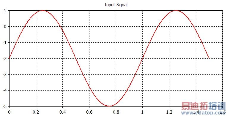
Pic 1: Original signal (DC-shifted sine wave)

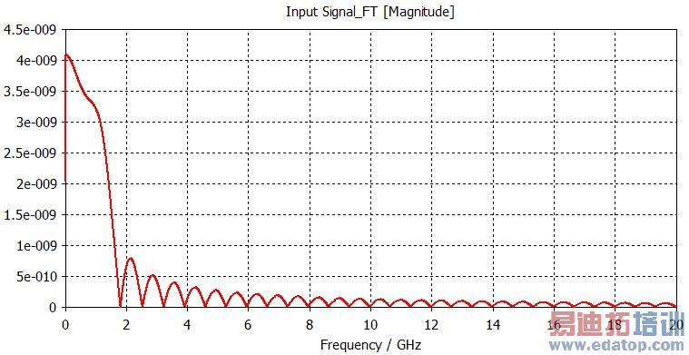
Pic 2: and its FT:

Inverse Fourier Transform (IFT)

This option calculates the Inverse Fourier Transform of the input function, specified in the "1D Results" box. The user has the option of either defining one (complex) input function, or two input functions: Magnitude and Phase. In the latter case, the two functions will be internally combined into one complex function before calculating the IFT.

The IFT will return a time signal between Tmin and Tmax, as specified by the user. If the 'Auto' option is used for Tmax, it will be set to 1/(2*Delta_f), where Delta_f is the frequency resolution of the input spectrum. The user may also enter the number of samples and a normalization factor. Please see the FT section for details about the choice of normalization. If the input spectrum contains positive frequencies only, the checkbox "From half-sided spectrum" should be checked.

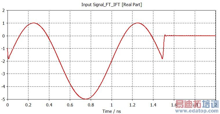
Pic 3: Signal after inverse FT. Please note the "cutoff" that happens if a time interval larger than the original is entered.

Fourier Series (FS)

This option calculates the complex-valued Fourier Series (FS) coefficients of a given function, as specified in the '1D Results' box.  In almost all cases, the input function will be real-valued. However, complex-valued input functions are allowed for completeness. The number of coefficients calculated is determined by the settings 'nmin' and 'nmax'. The FS represents a discrete series, with coefficients defined at discrete frequency points. Accordingly, the FS will be plotted in a spike-like pattern, where as the FT will show a continuous spectrum.

Like for the FS, the user may select to resample the input function with the Nyquist rate and to calculate a half-sided spectrum. For more details on these options, see the FT section above. The FS assumes the input signal to be periodic with a period of T0. If the 'Auto' option for the period length is active, the template will assume T0 to be the total length of the input signal. It is possible to use mathematical expressions in this textbox. For example, if two pulses were calculated, the user might enter "[Auto:Length of input signal]/2" in the 'Period of time signal' box.

The normalization settins are equivalent to the FT and IFT, see above for details. A normalization of '1' for both FS and IFS will ensure FS(IFS(f)) = f.

The 'Result type' option allows to generate a fully complex result, or to generate magnitude and phase separately.

Original signal (DC-shifted sine wave)

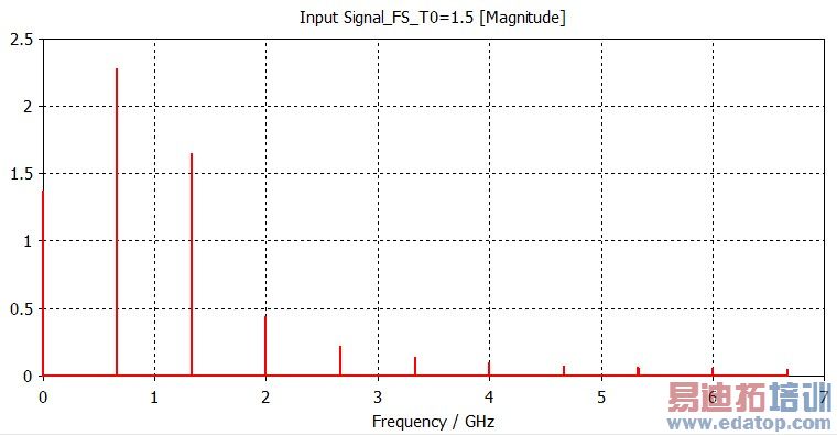
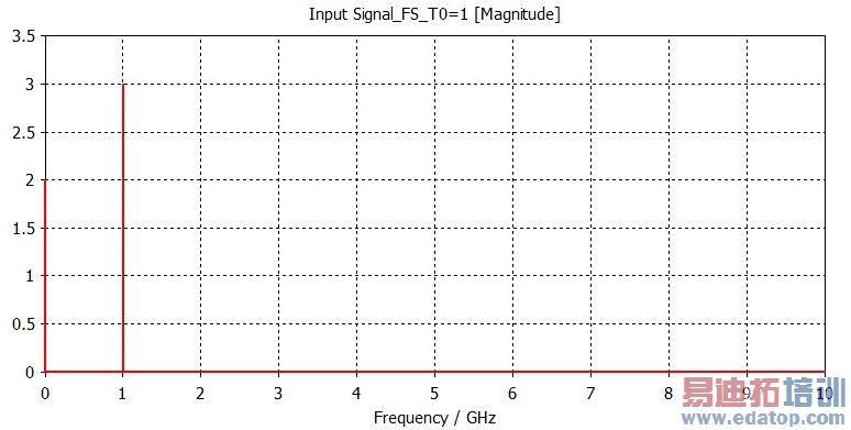
Pic 4:FS with T0=1.5

Pic 5:FS with T0=1

Inverse Fourier Series (IFS)

This option recreates a continuous, periodic time signal from the coefficients of the Fourier Series. The input function containing the complex-valued coefficients can be selected in the '1D Results' box.  The user has the option of either defining one (complex) input function, or two input functions: Magnitude and Phase. In the latter case, the two functions will be internally combined into one complex function before calculating the IFS.

The IFS will return a time signal between Tmin and Tmax, as specified by the user. If the 'Auto' option is used for Tmax, it will be set to 1/Delta_f, where Delta_f is the frequency resolution of the input spectrum. The user may also enter the number of samples and a normalization factor. Please see the FT section for details about the choice of normalization. If the input spectrum contains positive frequencies only, the checkbox "From half-sided spectrum" should be checked.

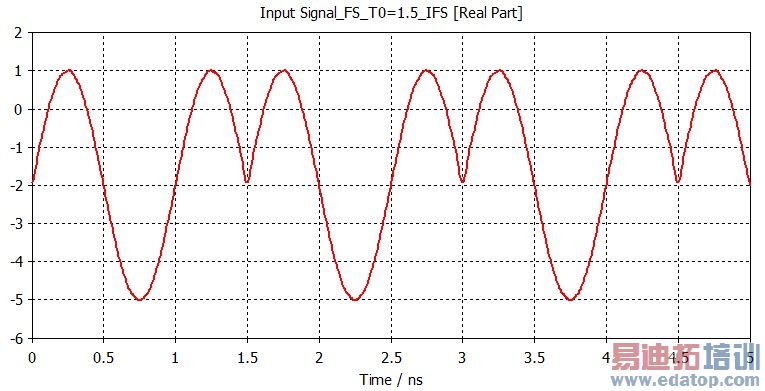
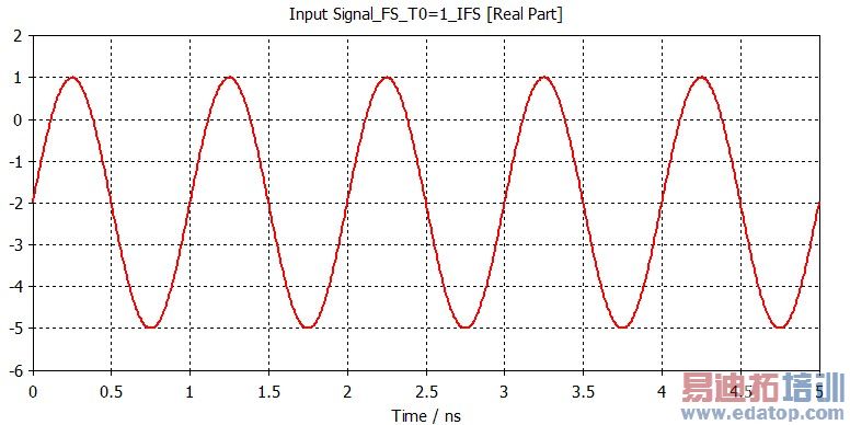
Pics 6 and 7: Recreated, periodic time signals from FS with T0=1.5 and T0=1, respectively. There is no cutoff this time, the signal will be continued periodically with T0.

Power Spectrum Density (PSD)

This option calculates the Power Spectrum Density distribution of the input signal between Fmin and Fmax, as specified by the user. The input function can be selected in the '1D Results' box. Entering a complex-valued input function is possible, but only the real part of the input function will be considered in this case. The PSD distribution, a real-valued function, is given in dB and is normed to a maximum value of 0 dB.