CST2013: Frequency Domain Solver Problem Handling

This page contains a list of the most important warning messages together with a detailed explanation of the meaning and proposal for handling and resolution.

Farfield monitors have been defined. Please consider changing the solver settings for open boundaries to improve their accuracy.

The message is displayed by the Frequency Domain Solver with tetrahedral mesh if farfield monitors and "open" or "open (add space)" boundary conditions are defined. Different kinds of open boundaries are available for the solver. Each realization of the open boundary condition has its particular advantages and disadvantages. The default "standard impedance boundary condition" provides results at low computational costs. In order to increase the accuracy, other choices are available in the solver specials. Please consider enabling the "add space before mesh generation" option, which adds more surrounding space to increase the distance from the structure to the open boundary even beyond the visible bounding box with "open (add space)" boundary conditions. Even higher accuracy (lower artificial reflection at the open boundary) can be obtained at higher computational cost by using the PML. See the section Open boundary frame in the solver specials for further details.

The S-parameter error threshold value ("xxx") is smaller than the desired linear equation system solver accuracy ("yyy").
It is recommended to use an S-parameter error threshold value (currently set to "xxx") which is ... larger (for instance "XXX") than the desired linear equation system solver accuracy ("yyy").
It is recommended to use a linear equation system solver accuracy (currently set to "yyy") which is ... lower (for instance "YYY") than the desired S-parameter error threshold value ("xxx").

One of the three recommendations is displayed (the first condition is considered as an error in the setup) if the relation between two accuracy settings of the solver needs to be improved: first of all, the linear equation system solver's relative residual threshold "yyy" (referred to as "Accuracy" in the Solver settings frame of the Frequency Domain Solver Parameters, and second, the broadband sweep's convergence threshold "xxx", see the S-parameter error threshold value in the Frequency Domain Solver Sampling dialog.

Please follow the proposal displayed in the text or choose an even lower threshold for the linear equation system solver's accuracy. If you change the settings accordingly, the broadband frequency sweep possibly requires fewer frequency samples. Usually this results in an increased overall solver performance.

Similar statements hold, as an example, for the S-parameter threshold of the adaptive mesh refinement. It should be chosen good enough for the broadband frequency sweep, but no better than the linear equation system solver's accuracy setting allows.

There are large gaps between some frequency sampling interval definitions: ...

This warning is displayed if frequency sampling intervals have been defined with some "gaps" where the solver is not allowed to place new automatically chosen frequency samples. Please check your settings in the Frequency samples frame of the Frequency Domain Solver Parameters dialog.

For instance, in a global frequency range from 5 to 10 GHz, imagine that two sampling intervals have been defined: the first one from 5 to 7 GHz and the second from 9 to 10 GHz. The solver can place new frequency samples in those intervals only. The S-parameter values in the "gap" from 7 to 9 GHz are then influenced by the frequency samples in the two intervals only. Hence, the S-parameter sweep may fail to converge, or: the S-parameter's accuracy might be low in these "gaps" of the global frequency range. It is recommended to run two simulations in that case, one for each interval individually.

A second example is if there is only one automatic frequency sampling interval and one automatic adaptive mesh refinement sample that is not contained by the automatic frequency sampling interval. With the global frequency range of 5 to 10 GHz as an example, the default mesh adaptation frequency will be 10 GHz. Now if the automatic frequency sampling interval is limited to the range 5 to 7 GHz, there is a "gap" from 7 GHz to the adaptation frequency at 10 GHz. In that case, please move the mesh adapatation frequency into the interval.

The input reflection of the S-parameters seems to be large at "xxx". The adaptive mesh refinement at this sample will be stopped. A new mesh adaptation frequency has been added ... at "yyy"
The input reflection of the S-parameters seems to be large at "xxx". A constant mesh adaptation sample will not be changed.
The input reflection of the S-parameters seems to be large at "xxx". The lowest and highest mesh adaptation samples in an adaptive sampling interval must be calculated for the broadband sweep.
The mesh adaptation sample will not be moved again. Please define a suitable constant adaptation frequency.

Those messages or warnings are displayed in the context of the adaptive mesh refinement. For the sake of accuracy, it is important to have a mesh adaptation sample at some frequency where power is delivered into the structure, for instance in the passband of a filter. If the mesh adaptation frequency is defined at a frequency where most of the input power is reflected, the error indicator will not "see" the possibly more important interior parts of the structure, and the mesh refinement will focus on the terminals of the structure rather than refining in the inner regions.

The solver may therefore stop the adaptive mesh refinement if the minimum input reflection of all S-parameters at the present adaptation frequency seems to be too high. It attempts to insert new adaptation frequencies with a trial-and-error approach that covers the whole frequency range, starting with monitor frequency samples, if any. The number of attempts to "move" the automatic adaptation frequency samples is limited. If no suitable frequency is found, the adaptive mesh refinement will continue at the first adaptation frequency again. In this case, please choose and define a suitable constant adaptation frequency in the Frequency samples frame of the Frequency Domain Solver Parameters dialog.

Mesh adaptation samples which are not defined as "Automatic" and hence are constant will not be moved, for instance single frequencies or equidistantly spaced samples. If an "Automatic" sampling interval definition has more than two samples, its lowest and its highest frequency will be calculated in any case because the S-parameters at those frequencies are required for the broadband frequency sweep.

A completely shielded, separated region was found near ...
Completely shielded, separated regions were found near ...

The solver has detected that regions exist which are not electrically connected to any other part of the model. This often is an unwanted side effect of the modelling. If the regions are separated and solved one at a time, or if a small cavity can be "filled", the structure is simplified and thus easier to solve. An isolated region which does not contain any source is free of fields and can be filled by perfect electric conducting (PEC) material without changing the solution.
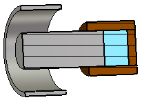
As an example, a coaxial line (gray) is sketched, the inner conductor of which is plugged into some socket (brown). This leaves a vacuum cavity between the inner conductor and the socket, which is highlighted in light blue in this illustration.
Please consider removing this cavity for instance by adding a PEC inset.

As an alternative to the fast resonant solver's adaptive mesh refinement, please consider running the solver automatically after the general purpose solver's adaptive tetrahedral mesh refinement.

This hint is displayed for the fast resonant Frequency Domain solver with tetrahedral mesh to refer to a way to combine the general purpose solver's adaptive tetrahedral mesh refinement with the fast resonant solver. Instead of running the fast resonant solver directly with its own mesh refinement, there is an option to run the fast resonant solver after the general purpose solver's mesh refinement:

Switch to the "General Purpose" Method in the corresponding frame of the Frequency Domain Solver Parameters. Click on Properties... next to Use broadband frequency sweep (enable if necessary) to bring up the Frequency Domain Solver Sampling dialog.

Enable Run after adaptive mesh refinement if applicable in this dialog to let the general purpose solver stop after the adaptive mesh refinement without performing the interpolative sweep. Afterwards, the fast resonant solver method will be executed to calculate the broadband results. This is an alternative and efficient way of using the fast resonant solver method, especially if the faster single point adaptive mesh refinement of the general purpose method is preferred.

If a required feature prevents the fast resonant solver from being applied, the default interpolative sweep is used. The solver log file provides a hint about the missing features, which possibly can then be removed (for instance, some field monitors which are unsupported by the fast resonant solver.)

Most of the prerequisites have been checked if this message is displayed. There is one possible exception for those cases where the port mode calculation detects modes other than TEM, TE, or TM. The fast resonant solver will still be used for the sweep in that case (in order to avoid those modes being approximated, please turn off Run after adaptive mesh refinement if applicable to force the interpolative sweep.)

Performing parallel excitation with "xxx" threads.
Performing block parallel excitation with "xxx" threads.

This information is displayed when the iterative solver is used with up to "xxx" excitations calculated in parallel. While the direct solver usually benefits from all the cores available on the CPUs in the computer and thus uses as many threads as cores are available, the iterative solver may choose to use less threads. This is because of mainly two reasons: the memory requirements for the parallel computation of excitations increase with the number of excitations, and the memory bandwidth of the computer may limit the number of parallel excitations for which an increase of performance is seen.

The default number for "xxx" is twice the number of sockets in the computer, and was found to be a good choice for many hardware architectures.

However, advanced users can overwrite the behavior of the parallel iterative calculation of excitations by calling the "SetCalculateExcitationsInParallel" method of the FDSolver object. See the Visual Basic (VBA) Language online help for details.

As the iterative solver is running in parallel for up to "xxx" excitations at the same time, there is no text output of the relative residual norm per excitation into the message window. But the progress of the iterative solver can be accessed in the Navigation Tree, see "1D Results/Convergence/Solver/Residuals".

S-parameter ports are not defined.
Therefore, the adaptive mesh refinement will stop after the maximum number of passes ("xxx").
Furthermore, frequency sample definitions without an explicitly given number of samples cannot be considered.

These messages are for instance shown with plane wave excitation only.

S-parameter results are used as a stopping criterion for the adaptive tetrahedral mesh refinementin the general purpose frequency domain solver. In the course of the interpolative broadband frequency sweep, the choice of "automatic" frequency samples is based on S-parameters, too.

Thus, if no S-parameters are defined, the solver will by default stop if themaximum number of adaptive mesh refinement passes is reached. However, any kind of 0D result template can be used as a stopping criterion with a few modifications of the solver's mesh adaptation properties: First define a result template which extracts a 0D result, for instance the magnitude of the electric field at some location (see the Template Based Post Processing Overview for details.) Then open the Adaptive Tetrahedral Mesh Refinement properties. Deactivate the criterion "S-parameter" below "Check at discrete adaptation samples."Activate the "0D Result Template..." below "Check after broadband calculation" instead and choose the result template from the drop down list. If required, change the relative threshold and the number of checks. The solver will thenuse the 0D result template as a stopping criterion for the adaptive mesh refinement.

"Automatic" frequency sample definitions are ignored if no S-parameter results are generatedduring the simulation. For plane wave excitation this usually means that all frequencies of the field monitors will be calculated,and no additional frequency samples are placed elsewhere unless the sampling definition is changed to "single", "equidistant", or "logarithmic", as described in the Frequency Domain Solver Overview.