- 易迪拓培训,专注于微波、射频、天线设计工程师的培养
CST2013: Field Source Overview
录入:edatop.com 点击:
Several types of field sources are available for imprint in CST MICROWAVE STUDIO:
Plane wave sources allow for the efficient excitation of linear, circular or elliptical plane waves at the boundary of the calculation domain.
Farfield sources allow for the excitation of the integral equation solver and the asymptotic solver by data exported in a farfield source file by CST MICROWAVE STUDIO.
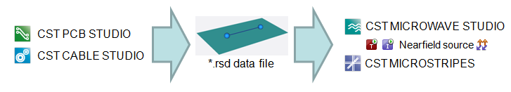
Nearfield sources allow for the excitation of the transient solver by FSM nearfield data recorded with field source monitors in CST MICROWAVE STUDIO, by RSD current distributions calculated by CST CABLE STUDIO or CST PCB STUDIO, and by external formats as NFD radiation data exported e.g. from Sigrity® tools or NFS nearfield scan data exchange format.
Plane Wave Source 
The plane wave excitation source provides you the opportunity to simulate an incident wave from a source, located a large distance from the observed object. In combination with farfield monitors, the radar cross section (RCS) of a scatterer may be calculated.
Please note that the input signal of an excited plane wave is normalized due to the user-defined value of the electric field vector (unit: V/m). The phase reference location of the plane wave excitation is the origin of the calculation domain.
When exciting with a plane wave, several conditions must be satisfied, which will be discussed in the following section.
Note: In case of plane wave excitation onto an infinite periodic structure, the unit cell approach is recommended, which is accessible via the boundary dialog.
Boundaries and background material
When exciting with a plane wave, several conditions must be satisfied. First, open boundary conditions must be defined at the direction of incidence.
In the picture below, a plane wave is passing the calculation domain in the (1, 1, 1) direction. At a minimum, the boundaries at xmin, ymin and zmin must be defined as open boundaries (for an undisturbed propagation, xmax, ymax and zmax must be open as well).

When using a plane wave source, other excitation ports must not be located on boundary conditions. Moreover the surrounding space should consist of a homogenous material distribution. This implies that the background material is set to a normal, not a conducting material.
Decoupling plane
If the calculation domain is intersected by a metallic plane which is supposed to extend to infinity, it is necessary to define this structure as a decoupling plane. Any PEC plane touching the boundaries is automatically detected as a decoupling plane. In case of a failed or erroneous detection it is possible to define a decoupling plane manually in the Plane Wave dialog. Only decoupling planes aligned with the cartesian coordinate axes are supported. Please add space at the boundaries if the simulation of a finite PEC structure is intended.
A decoupling plane restricts the plane wave excitation to the front domain and includes the reflected wave properly in the excitation. The picture below illustrates the effect of a decoupling plane (marked with a pink frame) in a 3D simulation. A typical interference pattern is visible behind the plane. Moreover, a decoupling plane also influences the RCS of a structure. The RCS of an infinite PEC plane is zero by definition, as the reflected wave is an integral part of the excitation. Hence only additional features are visible in the RCS (e.g. the slots in the example below).
Polarization
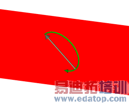
It is possible to define three different kinds of polarizations for a plane wave excitation: linear, circular or elliptical. For linear polarization, one electric field vector exists for the excitation plane with a fixed direction. This electric field vector changes its magnitude according to the used excitation signal. A linear polarization is displayed as red plane with a green electric field vector and a blue magnetic field vector. The visualization of the linear plane wave excitation is displayed in the picture below.

For circular or elliptical polarization, two electric field vectors exist in the excitation plane perpendicular to each other. Each of these two vectors define one linear polarized plane wave. If these two linearly polarized plane waves are excited simultaneously, the resulting plane wave is elliptically polarized. Please note that circular polarization and linear polarization are special cases that may result from the definition of an elliptical polarization.
For a circular or elliptical polarization, the two electric field vectors are excited simultaneously according to the excitation signal with a certain time delay. This time delay is calculated for a given reference frequency and a phase shift between the two electric field vectors. In addition, the magnitude of the two electric field vectors may be different. The axial ratio defines the ratio of the magnitudes between the defined (first, primary) electric field vector and the perpendicular second vector.
The special case of a linearly polarized plane wave excitation is obtained if the phase shift between the two electric field vectors is 0 or 180 degrees. Please note that the phase shift is always related to the given phase reference frequency.
For a circular polarization the axial ratio is always 1 as well as the phase shift is always +90 or -90 degrees. Therefore, only two possible configurations exist for a circular polarization: left and right circular polarization. The circular polarization is displayed as a green circular arc starting at the primary electric field vector (gray color) using an arrow to indicate whether left or right circular polarization is used. The visualization of a left and right circular plane wave excitation is displayed in the two pictures below.
|
|
Left Circular Polarization (LCP) | Right Circular Polarization (RCP) |


If the phase shift differs from +90 or -90 degrees or the axial ratio is not equal to 1, the polarization is elliptical. Elliptical polarization is displayed similar to circular polarization. An elliptical arc denotes the sense of the polarization and its magnitude in the plane regarding the course of time at the given reference frequency. The arc starts at the resulting electrical field vector at the time when the primary electric field vector (i.e., the field vector of the first linear plane wave) is at maximum. This resulting field vector is displayed as a green arrow if there is a significant difference to the primary field vector (gray).
If the phase shift at the reference frequency is positive, the time when the primary field vector reaches its maximum equals a phase of 0 degrees for an electric field monitor defined at the reference frequency. If the phase shift is negative, there will be an additional phase offset between the fields recorded by an electric field monitor at the reference frequency and the green arrow will be visualized when the plane wave definition is visualized.
The visualization of three different elliptical plane wave excitations is displayed in the three pictures below.
|
|
|
Axial ratio: 0.6667 | Axial ratio: 1 | Axial ratio: 0.6667 |


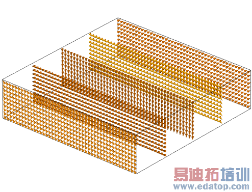
The following picture shows the spatial field distribution of a plane wave excitation with right circular polarization for a fixed time. Please note that for a fixed time, the spatial rotation of the field along the propagation direction is in the left direction for a right circular polarized plane wave.
Farfield source 
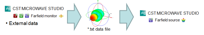
Farfield sources are available as excitation for the Integral Equation Solver or the Asymptotic Solver and are set up via the Farfield source dialog. The required farfield source data can be exported from results recorded by Farfield monitors by selecting Post Processing: Exchange Import/ExportExportFarfield Source. Alternatively, external data can be written in the farfield source file format and imported. The following diagram illustrates this workflow:
A farfield source does not act only as an excitation, but is also able to receive radiation. Hence S-parameters and F-parameters are calculated as well under the assumption of a perfectly matched antenna (i.e. a single farfield source in free space has an S-parameter equals zero).
A complete description of the farfield source file format can be found here.
Nearfield source 
Nearfield sources can be imported via the field source dialog. Available import formats include RSD current distributions from CST CABLE STUDIO and CST PCB STUDIO, FSM nearfield source data from CST MICROWAVE STUDIO, and NFD radiation source data from external sources, e.g. from Sigrity
All nearfield sources are imported as frequency domain data. For the imprint in the CST MICROWAVE STUDIO integral equation solver, the data is interpolated at the excitation frequency. In the CST MICROWAVE STUDIO transient solver and the CST MICROSTRIPES TLM solver, the data is imprinted via the broadband imprint.
Broadband imprint
For the imprint in the CST MICROWAVE STUDIO transient solver and the CST MICROSTRIPES TLM solver, this data is transformed into the time domain by an especially filtered inverse Fourier transform. This transformation is designed to produce optimal results for frequency domain monitors; the produced time domain signal and any time domain monitors do not directly represent meaningful data. Also, this transformation produces most accurate results at the discrete sample frequencies of the input data; for frequencies in between, an interpolation is required. Any data for DC, i.e. frequency 0, is disregarded.
Note: The duration of the excitation signal is inversely proportional to the frequency sampling rate of the imported data (due to the underlying inverse Fourier transform). To reduce simulation time, the frequency sampling rate can be down-sampled during the import of nearfield sources in the field source dialog.
Note: During the excitation of the broadband source in the CST MICROWAVE STUDIO transient solver, the recorded excitation signal will show an arbitrary value of 1. E.g. for a nearfield source with the name "fs1," the excitation signal might look like this:
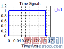
Note: The input data of nearfield sources is considered to be complex peak amplitudes of the currents or fields. No normalization of the input data is performed. Thus any frequency domain monitors directly show the resulting quantities for an excitation with the current or field data given in the imported file.
Note: Due to the use of an inverse Fourier transform, the input frequency samples must always correspond to an "equidistant - zero frequency base" sequence:
The term "equidistant" means that the frequency sampling should be equidistant.
The term "zero frequency base" means that the sequence of frequency points must exactly hit the zero frequency when extending equidistantly at the lower frequency end.
As an example, if the imported file contains the frequency samples
0, 1, 2, 3, 4, 5, 6, 7, 8, 9, 10, 11, 12, 13, 14, 15
the frequency sequence obtained with Downsampling ratio=4
4, 8, 12
is an equidistant - zero frequency base sequence, whereas
3, 7, 11
is still equidistant but not any more zero frequency based (extrapolating the sequence using frequency step=4 does not hit the 0 frequency value).
Equivalence principle
Using nearfield source monitors, one can represent parts of a model including excitation by replacing these parts with nearfield sources. The equivalence principle assures that fields outside of these parts do not change if the model outside does not change either.
A standard use of nearfield sources requires one to change the model outside of the nearfield source region, though: E.g. one simulates a radiating device in free space, monitors the nearfields on a box, and imprints it in a new model where an additional scatterer is included. Strictly speaking, there is no guarantee that the fields and derived quantities for this new model resemble the results of a direct simulation of the radiating device with the scatterer. As long as the coupling to the radiating device is weak, very good results can be achieved by this approximation, though. To improve the results of the new model, one can approximate the first order effects of the coupling by replacing the radiating device in the nearfield source region by an approximate model.
These concepts will be illustrated in the following by a horn antenna example and an additional dielectric scatterer.
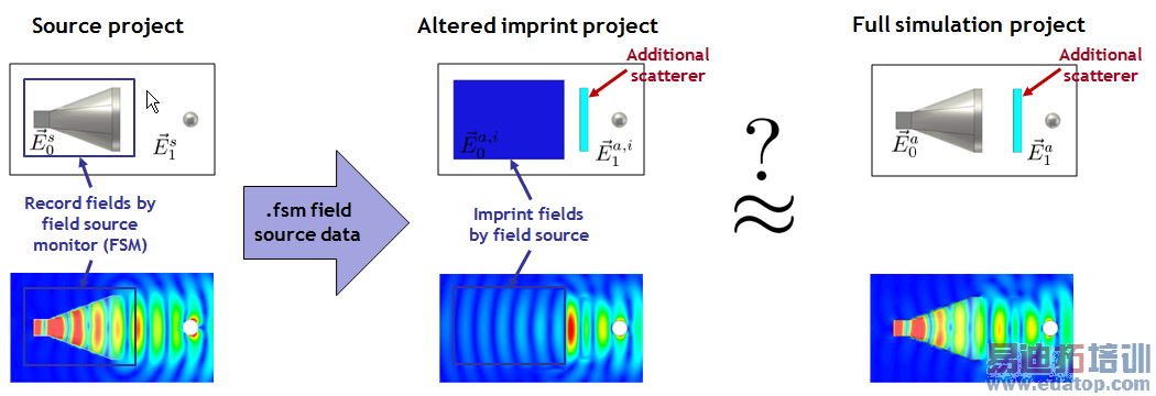
Take for example a horn antenna excited at a waveguide port with a metallic scatterer as the source project. If one places a field source monitor around the antenna and imprints the recorded data in an imprint project while keeping the metallic scatterer outside of the source region at the same position, the resulting fields E1 outside of the source region are the same for both projects. The fields E0 inside of the source region are zero in the imprint project. Therefore, the imprint project could be changed arbitrarily inside of the source region without changing the results. Good agreement of the outside fields and almost zero fields in the source region (up to numerical artifacts) can be seen in the following example:

This calculation without changing the imprint project outside of the source region is not very useful, though, as the fields outside the source region and derived quantities are already known from the simulation of the source project. As mentioned above, one can now try to approximate a full simulation project (here by adding a dielectric scatterer outside of the source region) by imprinting the field source of the source project in an altered imprint project. Whether this approximation is reasonable depends on the problem at hand. For the addition of the example dielectric scatterer, the results of the altered imprint project agree reasonably well with those of the full 3D simulation of the full simulation project (outside of the source region):
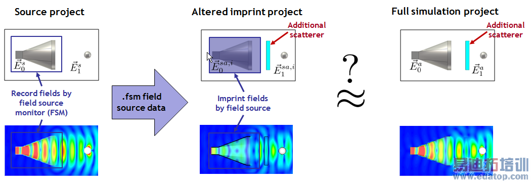
In the above altered imprint project, one notices that fields are scattered back to the source region, though. These would normally interact with the source structure. To approximately account for the interaction of these fields with the horn antenna, one can now put the horn antenna structure (or usually an approximation) inside the source region. In the following example, one can discern slight improvements of the approximation of the fields outside of the source region:
A note on the spatial interpolation: The imported data contains field values at a specific spatial discretization. Since this discretization does not match the one used in the simulation, the field values are interpolated between the original and the simulation grid. Due to this, a sufficiently fine simulation grid on the imprint box in the source project and the imprint project is recommended for accurate simulations. The energy-based mesh adaptation is a good choice for automatically adapting the grid in the imprint project; alternatively, local mesh properties can be set for nearfield sources.
RSD current distribution
RSD current sources can be created by CST CABLE STUDIO or CST PCB STUDIO. The creation of these sources is activated in the AC simulation task settings in CST DESIGN STUDIO. Sources stemming from CST CABLE STUDIO can be imprinted in both time domain solvers (hexahedral and hexahedral TLM), in the integral equation solver of CST MICROWAVE STUDIO and in the TLM solver of CST MICROSTRIPES (see RSD current source). Sources stemming from CST PCB STUDIO can only be imprinted in the transient solver of CST MICROWAVE STUDIO. Please note the description of the broadband imprint.
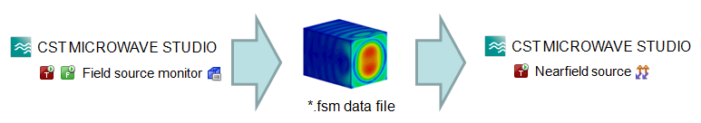
FSM nearfield source
FSM nearfield sources can be recorded by the hexahedral transient solver and the tetrahedral frequency domain solver of CST MICROWAVE STUDIO by defining a field source monitor. The resulting FSM nearfield source files can be found in the results folder of the original project. The FSM nearfield sources can be imprinted in the CST MICROWAVE STUDIO transient solver, the hexadral TLM solver supports the data from the hexadral transient solver. Please note the description of the broadband imprint and the equivalence principle.
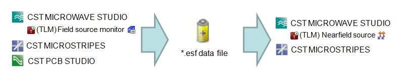
ESF compact source
ESF compact sources can either be created by the TLM solver of CST MICROWAVE STUDIO or of CST MICROSTRIPES as well as by CST PCB STUDIO. They can be imprinted in the TLM solver of CST MICROWAVE STUDIO or CST MICROSTRIPES (RSD current source).
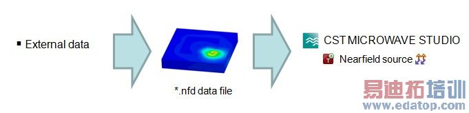
NFD radiation source
NFD radiation sources describe the equivalent surface fields on a box, similar to the FSM nearfield sources. They are for example provided by Sigrity
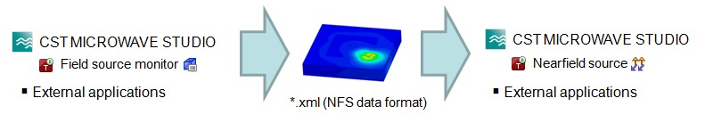
NFS nearfield scan data exchange format
Similar to the NFD file format, the NFS file format allows the imprint of equivalent surface fields on a box or even on single planes. This format is especially designed for scan data and is able to handle an equidistant as well as a non-equidistant sampled spatial distribution of field data.
The format is based on the IEC? Technical Report IEC/TR 61967-1-1. In order to describe surface fields on a rectangular box surface, each face and field component has to be defined in a single XML-file and a corresponding DAT-file.
The XML-file contains all meta-data such as field type, field components (Ex, Ey,Ez, Hx, Hy, Hz ), frequencies, and a reference to the DAT-file.
The DAT-file contains the actual field data values in the following ASCII pattern:
x0 y0 z0 Re(freq1) Im(freq1) Re(freq2) Im(freq2) Re(freq3) Im(freq3) ...
x1 y0 z0 Re(freq1) Im(freq1) Re(freq2) Im(freq2) Re(freq3) Im(freq3) ...
x0 y1 z0 Re(freq1) Im(freq1) Re(freq2) Im(freq2) Re(freq3) Im(freq3) ...
...
Where (x_i, y_j, z_k) describe point positions of a cartesian grid and Re(freq1)/ Im(freq2)the real/imaginary part of the field value at frequency freq1 and position (x_i, y_j, z_k).Example files for the supported types of the NFS format for the CST MICROWAVE STUDIO transient solver can be found here. A detailed description of the file syntax can be found in IEC? Technical Report IEC/TR 61967-1-1.
Field source monitor export as NFS nearfield scan data exchange format
In order to export data of a field source monitor it is necessary to convert an existing FSM file into the desired NFS nearfield scan data exchange format. This can be achieved in two ways with a VBA command:
1. Directly by absolute path to an existing FSM file:
'creates a folder "c:dummymy_monitor_file" in the parent folder of an existing FSM file with a set of NFS files.
With Monitor
.Reset
.Export ("nfs" ,"" ,"c:dummymy_monitor_file.fsm", True)
End With
2. Indirectly by the name of the field source monitor and the excitation name used:
'creates an additional folder in the result folder of the current project with an existing FSM file: "$PROJECT_RESULT_FOLDER$$FIELD_SOURCE_MONITOR_NAME$_$EXCITATION_NAME$".
'E.g. "c:project_1Resultfield-source (f=4..6(3))_5": where $FIELD_SOURCE_MONITOR_NAME$ is "field-source (f=4..6(3))", $EXCITATION_NAME$ is "5" if port "5" was excited and $PROJECT_RESULT_FOLDER$ is "c:project_1Result".
'This folder will contain a set of NFS files.
With Monitor
.Reset
.Name ("field-source (f=4..6(3))")
.Export ("nfs" ,"5" ,"", True)
End With
'In case of a simultaneous excitation the excitation name is exactly the string in the "Label" field of the Excitation Selection Dialog. E.g. "2[1.0,0.0]+3[1.0,0.0]"
With Monitor
.Reset
.Name ("field-source (f=4..6(3))")
.Export ("nfs" ,"2[1.0,0.0]+3[1.0,0.0]" ,"", True)
End With
CST微波工作室培训课程套装,专家讲解,视频教学,帮助您快速学习掌握CST设计应用
上一篇:CST2013: Thermal Stationary Result Overview
下一篇:CST2013: Drag and Drop
CST培训课程推荐详情>>
 最全面、最专业的CST微波工作室视频培训课程,可以帮助您从零开始,全面系统学习CST的设计应用【More..】
频道总排行
- CST2013: Mesh Problem Handling
- CST2013: Field Source Overview
- CST2013: Discrete Port Overview
- CST2013: Sources and Boundary C
- CST2013: Multipin Port Overview
- CST2013: Farfield Overview
- CST2013: Waveguide Port
- CST2013: Frequency Domain Solver
- CST2013: Import ODB++ Files
- CST2013: Settings for Floquet B