CST2013: Farfield Overview

The farfield calculation deals with the field behavior far away from the corresponding source of the electromagnetic waves. At a sufficiently great distance compared to the regarded wavelength, respectively the dimension of the finite structure, the field components of a radiated or scattered field are approximately spherical waves. This means that higher order terms of 1 / r n, n = 2,3,... can be neglected and therefore mainly transversal field components exist - specifically, the theta and phi components referred to a basic spherical coordinate system.

The farfield components are derived from the calculated fields stored on the bounding box of the calculation domain. This is possible for different kinds of applications, but is primarily intended for the simulation of various antenna structures as well as the radar cross section of scattering problems. Furthermore, it is possible to consider the farfield of specific patterns of antenna arrays.

Radar Cross Section (RCS)

The radar cross section (RCS) is a farfield parameter that determines the scattering properties of a specific radar target. It represents a complex parameter depending on the incident wave (polarization, propagation angle, operation frequency) and the target itself (geometry, material characteristics). For the calculation of the radar cross section, you must define a farfield/RCS monitor as well as a plane wave excitation.

NOTE: The plotted RCS is the bistatic RCS for one incoming wave direction and all reflected wave directions. It is the monostatic RCS for only one farfield point that depends on the plane wave direction.

The RCS plot includes two integrated quantities which characterise the target:

Total RCS: The total radar cross section is defined as the ratio of the scattered power to the intensity of the incident plane wave.

Total ACS:  The total absorption cross section is defined as the ratio of  the absorbed power to the intensity of the incident plane wave.

Array Pattern

If you apply the pattern multiplication to a previously calculated farfield, the corresponding result for a specific antenna array built of identical elements can also be derived. The single antenna elements are defined by their position in space as well as their amplitude and phase information.

Farfield contribution of unit cells / periodic structures

A unit cell is the fundamental building block of a spatially periodic configuration such as a two-dimensional infinite array of antennas. Those arrays can be analyzed using periodic or unit cell boundary conditions. Please note that these boundary conditions will simulate a simultaneous excitation of all elements in the spatially periodic array, where the element-to-element phase advance is given by the boundary conditions.

Strictly speaking, the farfield result does only apply for an infinite array, which yields farfield contributions only for a discrete set of directions. However, the definition of a finite farfield array in the farfield postprocessing still provides useful results for sufficiently large (as compared to the single element) arrays. Thus the farfield of a single element might be misleading, as the accuracy of this approximation decreases with the number of array elements. This is in particular true for electrically small array elements.

The farfield calculation for periodic structures is performed by integrating an expression over the boundaries of the calculation domain. In this regard, there are two contributions to the farfield: The top (aperture-like) surface, which contributes most of the array radiation, and the sidewalls of the bounding volume which separate the individual array elements. Though the sidewalls do not contribute in the limit of an infinite array, they might provide a useful edge correction for finite arrays. It is possible to switch between the aforementioned two kinds of integration surfaces via the VBA command FarfieldPlot.IncludeUnitCellSidewalls. Please take a look at the VBA objects help page of the FarfieldPlot Object for details.

The following comment only applies to the Frequency Domain solver with tetrahedral mesh and unit cell boundary conditions: as the open boundary is realized by using analytic Floquet modes, an analytic expression is also available for the farfield integration of the Floquet port surface. The farfield calculation itself then can be deemed more accurate than the numerical farfield integration, and is faster. The latter however can only be true if the side-walls are excluded, since a numerical farfield integration has to be performed on the unit cell boundaries otherwise. Please note that for RCS calculations with the Frequency Domain solver, tetrahedral mesh and unit cell boundary conditions, side-walls are always excluded at the moment.

The results of the farfield calculations can be handled in the Farfield Plot Dialog offering different possibilities for visualizing: polar and Cartesian plots as well as 2D and 3D graphics. In each case, diverse components are available that are described in detail in the following, referred here to the electric field:

Farfield Components

A  farfield vector is composed of two tangential and one radial field component. These components are always ordered such that they form a right-handed coordinate system. Supported coordinate systems are:

Common components for all coordinate systems:

Absolute value: The absolute value of the electric field derived from the two tangential and radial component:

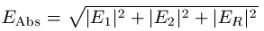   or with farfield approximation    

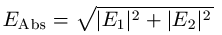
Radial: The radial component or the electric field ER.
Please note that this component is only available if the farfield is calculated without farfield approximation.

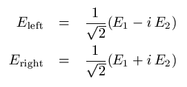
Circular polarization: Left and right polarized field components are calculated from the tangential components:

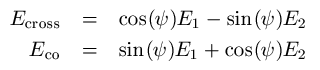
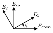
Slant polarization: Slant polarized field components are the tangential components rotated by an angle Psi :

Axial ratio: Following IEEE-Standard, the axial ratio is the ratio of the major axis to the minor axis of the polarization ellipse.  It is calculated as follows:

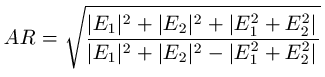
To avoid an infinite axial ratio caused by a minor axis of length zero, it is possible to plot the inverted IEEE axial ratio.

Phase: The phase is calculated using the real (Re) and imaginary (Im) part of a certain field component Ecomp as follows:

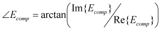
Please note that if the phase is plotted in 2D or 3D, the color ramp is set automatically to a special color ramp optimized for phase plots. In 3D plots the phase is plotted on the farfield surface.

Real part/Imaginary part: These cannot be plotted but are available through ASCII export or VBA commands.

Spherical:

Theta: The theta component of the electric field ET.

Phi: The phi component of the electric field EP.

Ludwig 2 Azimuth over Elevation: The theta and phi components of the farfield can be transformed to the "Ludwig 2 Azimuth over Elevation" representation. Please note that this transformation is usually performed with the main lobe aligned to the z'-axis (see Farfield Plot - Axes and Vertical and horizontal polarization). Therefore, the phi and theta angles below refer to the main lobe aligned coordinate system. The azimuth and elevation component are calculated as follows:

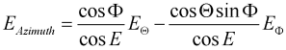
where

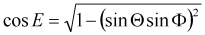
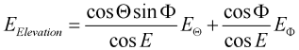
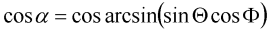
Ludwig 2 Elevation over Azimuth: The theta and phi components of the farfield can be transformed to the "Ludwig 2 Elevation over Azimuth" representation. Please note that this transformation is usually performed with the main lobe aligned to the z'-axis (see Farfield Plot - Axes and Vertical and horizontal polarization). Therefore, the phi and theta angles below refer to the main lobe aligned coordinate system. The alpha and epsilon component are calculated as follows:

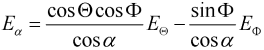
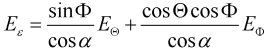
where

Ludwig 3: The theta and phi components of the farfield can be transformed to the "Ludwig 3" representation. Please note that this transformation is usually performed with the main lobe aligned to the z'-axis (see Farfield Plot - Axes and Vertical and horizontal polarization). Therefore, the phi and theta angles below refer to the main lobe aligned coordinate system. The vertical and horizontal component are calculated as follows:

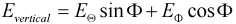
The field components of the afore mentioned coordinate systems are aligned with the cartesian coordinates:

Ludwig 3 components are not exactly aligned with the cartesian coordinate axes. The alignment given in the table above holds only for directions close to the z' axis.

Vertical and horizontal polarization: To analyze or visualize the vertical and horizontal polarization of the current farfield plot, some special settings concerning the rotation of the reference coordinate system may be made.

Some Farfield Terms

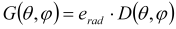
Directivity: The directivity of an antenna is defined as ”the ratio of the radiation intensity in a given direction from the antenna to the radiation intensity averaged over all directions.” The radiation intensity is given by the total power radiated by the antenna divided by 4p:

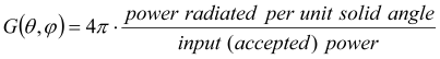
Gain: Accordingly, the gain is defined similarly but is related to the input or accepted power of the structure. In the case of a loss-free antenna (no conductional or dielectric losses), the gain is equal to the directivity. Note, that power flowing out any port is not considered as accepted by the structure.

Realized Gain: The realized gain is defined by gain * (1 - Balance^2), it includes the impedance mismatch loss.

E-field pattern: The electric-field pattern provides a distance-independent characterization of the radiation pattern. It is directly related to the electric field evaluated using the farfield approximation:

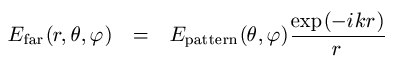
Due to its definition, the E-field pattern has the unit of a voltage.

Radiation efficiency: The antenna radiation efficiency is defined as the ratio of gain to directivity or equally the ratio between the radiated to accepted (input) power of the antenna:

or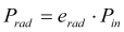

Total efficiency: The total efficiency is defined as the ratio of radiated to stimulated power of the antenna:

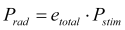
Compared to the input power, the stimulated power considers any occurring reflections at the feeding location.

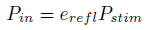
Reflection efficiency: The reflection efficiency is defined as the ratio of input to stimulated power. Note that the input power is the accepted power, i.e. reflected power and power flowing out any port of the simulated structure are not included.

Main lobe / side lobe: Radiation lobes are regions of the radiation pattern bounded by weak radiation intensity. The radiation lobe containing the direction of maximum radiation is termed main lobe or major lobe. All other lobes are termed minor lobes or side lobes.

Angular width: The angular width (or beamwidth) is defined as the angle between two directions where the radiation is dropped by 3 dB regarding the radiation in main lobe direction. This angle is located in a plane containing the main lobe direction .

Side lobe level: The side lobe level (or side lobe ratio) is the ratio of the power density in the side lobe to the power density in the major (or main) lobe. Here, the side lobe is the minor lobe with maximum intensity out of all minor lobes located outside the angular width.

Side lobe suppression: Inverse of the side lobe level.

Phase center: The phase center is defined as the reference point that makes the farfield phase constant on a sphere around an antenna. The phase center location depends on the plane and the radiation direction that is used for the phase center calculation. In addition, it depends on the polarization of an antenna as well. Please note that a unique phase center must not necessarily exist for an antenna.