- 易迪拓培训,专注于微波、射频、天线设计工程师的培养
CST2013: Discrete Port Overview
录入:edatop.com 点击:
Beside waveguide ports or plane waves, the discrete ports offers another possibility to feed the calculation domain with power. Two main port types are available: the discrete edge and the discrete face port. They are divided in three different subtypes, considering the excitation as a voltage or current source or as an impedance element that also absorbs power and enables S-parameter calculation.
Discrete ports are mainly used to simulate lumped element sources inside the calculation domain. These ports are a good approximation for the source in the feeding point of antennas when calculating farfields. In some cases, these ports may also be used to terminate coaxial cables or microstrip lines. However, due to the transmission between transmission lines of different geometric dimensions, reflections may occur that are much larger than those for the termination with waveguide ports. For lower frequencies (compared to the dimension of the discrete port), these reflections may be sufficiently small, such that these kinds of ports may also be used successfully for the S-parameter calculations of multipin connectors.
Please note that the input signal for the port is normalized depending on the chosen port type.
Discrete Edge Ports
General Description
Although the waveguide ports are the most accurate way to terminate a waveguide, discrete edge ports are sometimes more convenient to use. Discrete edge ports have two pins with which they can be connected to the structure.
This kind of port is often used as feeding point source for antennas or as the termination of transmission lines at very low frequencies. At higher frequencies (e.g. the length of the discrete port is longer than a tenth of a wavelength) the S-parameters may differ from those when using waveguide ports because of the improper match between the port and the structure.
Construction
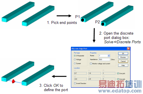
A discrete edge port consists of a perfect conducting wire connecting start and end points and a lumped element in the center of the wire.
The typical way to define a discrete port is to pick its two end points from the structure using the common pick tools and then to enter the discrete port dialog box:
Discrete ports can be applied to different types of port structures as presented below:
|
|
|
Coaxial port | Microstrip port | Coplanar port |
Note: The S-Parameter ports are the most frequently used Port Types and contain internal resistors for calculating S-Parameters with fixed reference impedances. In contrast, the Voltage and Current ports are ideal sources. The latter types of ports are normally used for EMC types of application.
Port Types
Voltage port: This port type realizes a voltage source, exciting with a constant voltage amplitude. If this port is not stimulated in the transient analysis, the voltage along the wire is set to zero. The voltage excitation signal will be recorded during the solver run.
Current port: This port type realizes a current source, exciting with a constant current amplitude. The current excitation signal will be recorded during the solver run.
Impedance element (S-Parameter type): This port type is modeled by a lumped element, consisting of a current source with an inner impedance that excites and absorbs power. The current source will only be active when the discrete element is the stimulation port in the transient analysis. This port realizes an input power of 1 W and enables the calculation of correspondent S-parameter, based on the incoming and outgoing time signals. In addition, it is also possible to monitor the voltage across and the current through the discrete port. Note that the orientation of the discrete port is used to determine the phase of the S-parameters.
Mesh Representation
The discrete port is defined by two points, determined either by picking two points or entering valid expressions for the point’s coordinates.
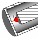
The input data can be seen in the Modeler View, where the discrete port is represented by a straight line and a cone. Due to the fact that discrete elements must be located on the calculation mesh, it is always advisable to examine the mesh representation of the element in the Mesh View. Here, one can observe that almost all elements on the grid consist of a metallic wire. Only the middle element contains the source.
Mesh representation of a discrete element, consisting of two metallic wires (marked in orange) and a source element (red cone). The colors of the wire and the cone can be changed in the Colors View Options dialog. |
|

Symmetry Planes
If a discrete port touches a symmetry plane, an electric plane must be chosen in the case of a perpendicular cut and a magnetic plane must be chosen in the case of a parallel allocation. The corresponding symmetry factors for the discrete elements will be considered automatically, such that the simulation results (depending on impedance and input power) will not be changed by the definition of symmetry planes. However, it should be mentioned that if an electric symmetry plane has been defined, the symmetry formulation varies slightly from the original problem regarding the element's allocation. As you can see in the picture below, the symmetric representation of a source directly at the symmetry plane is equivalent to a discrete element with two sources in the middle. Concerning the simulation results, this effect usually is negligible and can be ignored.

Discrete Face Ports
General Description
The discrete face port is a special kind of discrete port. It is supported by the integral equation solver, the transient solver, as well as the frequency domain solver with tetrahedral mesh. The discrete face port is replaced by a Discrete Edge Port if any other solver is chosen. Two different types of discrete face ports are available, considering the excitation as a voltage or as an impedance element which also absorbs some power and enables S-parameter calculation.
Construction
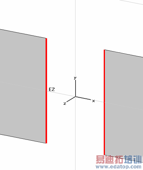
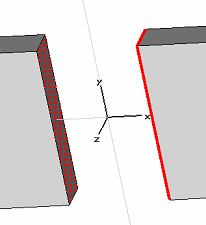
A face port can be defined by picking two separate edges (Pick Edge Mode) and choosing Simulation: Sources and Loads  Discrete Port. Further a discrete face port can be created between two edge chains. A surface will be created between an edge chain and a surface (Pick Face Mode) if one edge chain and one surface is picked.
|
|
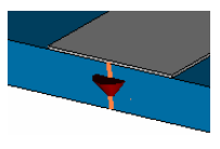
The face port will be created between the two selected edges. | Pick two edge chains, then add discrete port. |

|
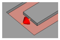
Pick an edge or an edge chain and a face, then add discrete port. |
|
|
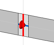
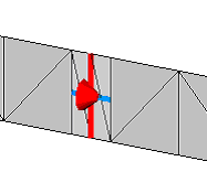
By default the excitation takes place at the (highlighted red) center edge of the port. A classical discrete port is also displayed. It will be used if another solver is used for simulation | The created surface is a PEC sheet and will be meshed. |
Port Types
Voltage port: This port type realizes a voltage source, exciting with a constant voltage amplitude. If this port is not stimulated in the transient analysis, the voltage along the wire is set to zero. The voltage excitation signal will be recorded during the solver run.
Impedance element (S-Parameter type): This port type is modeled by a lumped element, consisting of a current source with an inner impedance that excites and absorbs power. The current source will only be active when the discrete element is the stimulation port in the transient analysis. This port realizes an input power of 1 W and enables the calculation of correspondent S-parameter, based on the incoming and outgoing time signals. In addition, it is also possible to monitor the voltage across and the current through the discrete port. Note that the orientation of the discrete port is used to determine the phase of the S-parameters.
CST微波工作室培训课程套装,专家讲解,视频教学,帮助您快速学习掌握CST设计应用
上一篇:CST2013: Loss and Q Calculation Overview
下一篇:CST2013: Eigenmode Solver Overview
CST培训课程推荐详情>>
 最全面、最专业的CST微波工作室视频培训课程,可以帮助您从零开始,全面系统学习CST的设计应用【More..】
频道总排行
- CST2013: Mesh Problem Handling
- CST2013: Field Source Overview
- CST2013: Discrete Port Overview
- CST2013: Sources and Boundary C
- CST2013: Multipin Port Overview
- CST2013: Farfield Overview
- CST2013: Waveguide Port
- CST2013: Frequency Domain Solver
- CST2013: Import ODB++ Files
- CST2013: Settings for Floquet B