CST2013: Modeler View

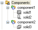
Components: In the navigation tree all components are displayed together with their associated solids. In order to distinguish single faces (solid2), from normal solids (solid1) and from mixed bodies (solid3), which include face and solid parts, all three types are indicated by different icons.

If a specific component is selected all its solids are visualized while the others are displayed transparently. If a single specific shape is selected, only this shape is visualized differently.

You can easily copy solids by means of the Copy and Paste Solids feature.

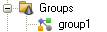
Groups: This is a convenient way to group objects (i.e. solids and wires) together. You can define 2 different kinds of groups i.e. Normal group   and Mesh group .

A normal group allows you to hide or show multiple objects at once. A mesh group offers the functionality of a normal group and in addition allows you  to define local mesh properties. Objects which are part of a mesh group inherits the local mesh properties from it. If there are multiple objects under a mesh group, they share the same local mesh properties.

An object cannot coexist in multiple groups of the same type i.e. It can be a part of a mesh group and a normal group at the same time, but cannot be a part of two different mesh groups or normal groups at the same time.

'Excluded from Simulation' and 'Excluded from Bounding Box' are two utility groups which are available by default. You can add objects to these groups, to exclude them from simulation or the bounding box.

Materials: If a specific material is selected all its solids are visualized while the others are displayed transparently.

Faces: In the navigation tree all faces are listed as green surfaces, in the main plot window they are also displayed in green. However, their color can be changed in the Colors View Options dialog.

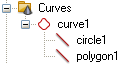
Curves: In the navigation tree all curves as well as their associated curve items (lines, circles, ellipses, rectangles, polygons, splines, 3D polygons)0 are listed. In the main plot window they are displayed in blue, however, this color can be changed in the Colors View Options dialog.

Wires: In the navigation tree all wires are listed as blue curves, in the main plot window they are highlighted in orange. However, their color can be changed in the Colors View Options dialog.

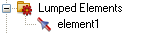
Lumped Elements: In the main plot window the lumped elements are shown as an orange line with a cone in their middle. However, their color can be changed in the Colors View Options dialog.

Plane Wave: It is only possible to define one plane wave as excitation signal. Selecting the corresponding  icon in the navigation tree visualizes the orientation of the field components and a red plane as the propagating wave front.

Ports: The discrete ports are plotted as an orange line with a red cone in their middle. Floquet ports are plotted by a red outline,  while waveguide ports are plotted in solid red. Their names (a number for waveguide and discrete ports) are show as well. In all cases the color of the ports can be changed in the Colors View Options dialog.

Field Sources: Field sources may be either imported current distributions or imported electric/magnetic field distributions. When the tree item is selected the location of the imported fields are plotted.

Farfield Sources: Selecting this item shows the spherical coordinate system used for the farfield source.

Excitation Signals: Excitation Signals describe the excitation function used for the transient stimulation of the defined sourcesport signals. Multiple signals , can be defined either manually or loaded from the Excitation Signal Library. A so called "Reference Signal" (indicated by the icon) is used as default stimulation in a normal transient solver run for stimulating the port modes, but performing a simulation with selected port modes and activated simultaneous excitation setting allows the stimulation of different ports with different excitation signals in one solver run.

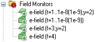
Field Monitors: All 2D monitors are visualized as a plane positioned at the specified location in the same color as their symbol in the navigation tree. Corresponding to this the 3D monitors are plotted as a colored wire frame box. This applies for the frequency monitors as well as for the time monitors.

Voltage Monitors: These monitors are visualized in the main plot window as a line or curve with a cone in the middle, all highlighted in dark green. However, this color can be changed in the Colors View Options dialog.

Current Monitors: These monitors are visualized in the main plot window as a line or curve with a cone in the middle, all highlighted in dark green. However, this color can be changed in the Colors View Options dialog.

Probes: The probes are shown as arrows with a point at the actual probe position in the same color as their symbol in the navigation tree.

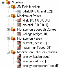
3D Field Monitors are used for the transient/time-domain solvers to compute a field in a given time frame. Each defined 3D Field Monitor will produce a vector field in the 2D/3D Results folder which can be animated over time..

Monitors at Points, Monitors on Edges or Curves, Monitors on Faces and Monitors on Solids or Volumes are indicated by a point, a line, a rectangle or a brick in the upper right corner of the icon, respectively. These monitors allow to observe certain physical quantities on different geometric entity and yield a real-valued scalar function (quantity vs. time) in the 1D Results folder.