- 易迪拓培训,专注于微波、射频、天线设计工程师的培养
CST2013: Power View
录入:edatop.com 点击:
Contents
1D power and loss curves
Power Accepted
Power Accepted per Port
Power Incident and Reflected
Power Stimulated
1D power and loss curves
| |
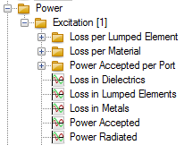
| Various 1d curves over frequency that show time averaged power spectra of sources and sinks of the electromagnetic field are collected in this folder. These contain the real part of the time average power dissipated in e.g. lossy materials and lumped elements. Furthermore, the power accepted from excited ports and the power radiated from the structure are shown. |

Power Accepted
| |
| Here, you may view the field energy over the time. The numbers in square brackets indicate the respective name of excitation. |
The accepted power is defined as the time average of the net power flow through the cross sectional area A of a port.
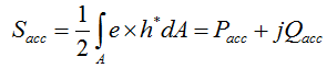
For every mode in a waveguide port or equivalently a discrete port excitation, this real power can be expressed in terms of forward (+) and backward (-) mode amplitudes c and the stimulating mode power p.
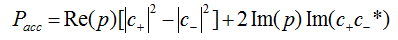
For waveguide ports considering more than one mode, the single powers per mode are added to yield the accepted power per port. (Please note that possible cross-coupling between the modes is neglected.) Finally, the real part of the sum of all accepted powers per port is shown.
Example: In this example, a horn antenna surrounded by open boundary conditions is considered. The structure is excited by a rectangular waveguide port over a broad frequency range.
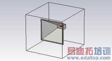
The power the structure accepted from the waveguide port almost completely radiates into free space.
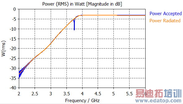
Notice that also for frequencies below the fundamental TE10 mode cut off (~3.75GHz), real net power is accepted by the antenna.
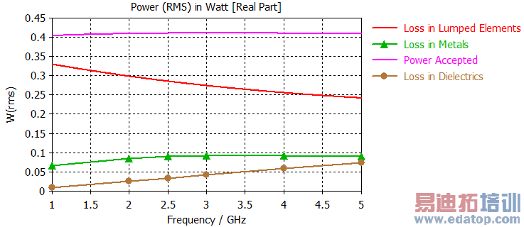
Example: In this example, different loss curves are shown for a microstrip line that is modeled by a lossy metal material. Furthermore, lossy lumped and face elements are contained that accept the power inserted by port 1.
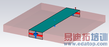
The sum of all losses equals the power accepted from port 1.
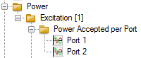
Power Accepted per Port
| |
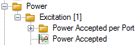
| In this sub folder, results for the accepted power for each port are stored. Ports that are not excited will show a negative accepted real power. |
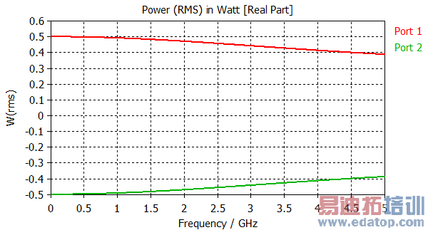
Example: In this example, a part of a microstrip line is considered. Both ends are terminated by a discrete face port. The excitation is performed via port 1.
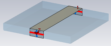
Since there are almost no reflections in the line, the real power that could be inserted by port 1 completely leaves through port 2.Notice that for time domain calculations the energy level must have decayed sufficiently in order to obtain this result.
Power Reflected
|
|
| The power that is reflected from the structure back into the source. |

The accepted power can be subtracted from the stimulated power (see below) to yield the reflected power.
It is calculated as the sum of the power that leaves the structure via all ports. Currently, only the real part of the reflected power is shown.
Power Stimulated
|
|
| The stimulated power shows the magnitude of the mode power p. For a loss-free waveguide port operating above the mode cut-off frequency this power would be inserted into the structure. |

CST微波工作室培训课程套装,专家讲解,视频教学,帮助您快速学习掌握CST设计应用
上一篇:CST2013: Smith Chart View
下一篇:CST2013: Probe Signal View
CST培训课程推荐详情>>
 最全面、最专业的CST微波工作室视频培训课程,可以帮助您从零开始,全面系统学习CST的设计应用【More..】
频道总排行
- CST2013: Mesh Problem Handling
- CST2013: Field Source Overview
- CST2013: Discrete Port Overview
- CST2013: Sources and Boundary C
- CST2013: Multipin Port Overview
- CST2013: Farfield Overview
- CST2013: Waveguide Port
- CST2013: Frequency Domain Solver
- CST2013: Import ODB++ Files
- CST2013: Settings for Floquet B