CST2013: Loss and Q Calculation Overview

Total losses of a simulated structure are accessible through a post-processing step, including dielectric losses as well as wall or surface losses. As a result of the loss calculation, the quality factor Q is available as well.

Volume losses

The volume loss power is calculated based on the normal material properties like the loss angle tangent delta or the corresponding conductivity and the field distribution in the corresponding shape volume:

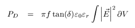
Note: The formula above delivers the average value of the dielectric loss power, whereas the input data contains peak values of the electric and magnetic fields.

This loss power is calculated in a post-processing step. However, material properties must be defined before starting a simulation as the solutions of the transient, frequency or JD(lossy) solver are influenced by these settings as well. In contrast, the AKS and JD(lossfree) eigenmode solvers do not take material losses into account. Nevertheless dielectric loss properties must still be defined before starting a solver to subsequently enable the loss and Q-factor calculation by a perturbation method.

Surface losses

The dissipated power due to surface losses is calculated by a perturbation method for all solver types. It is determined by  the specified conductivity, s, the permeability value and the magnetic field of a loss-free calculation:

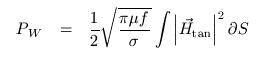
Note: The formula above delivers the average value of the absorbed power due to surface losses, whereas the input data contains peak values of the electric and magnetic fields.

This evaluation is accessible once the simulation has finished. Materials initially defined as PEC may be selectively set to a finite conductivity and a permeability value after the simulation run to customize the loss calculation. This includes single solid shapes as well as background and boundary materials (conducting enclosure). The loss calculation utilizes the magnetic field of a chosen mode (eigenmode solver) or the result of a previously defined 3D H-field monitor (transient and frequency domain solver). In contrast to dielectric losses, all material properties relevant for enclosure losses are set in the post processing.

Based on the results of the dielectric and the surface losses, the total loss energy is determined and separate values for the quality factor, Q, are deduced. Note that the electromagnetic field values are taken here without performing any further standardization.

For a better understanding in the following some further definitions are given:

Loss power

As mentioned, the total loss power

of the structure is the sum of dielectric and surface (including the boundary) losses.

Q-Factor

The quality factor, or Q-factor, is defined as 2 π times the ratio of the total energy W and the total loss power P divided by the period T:

The total energy is the entire amount of energy stored in the simulated structure, equal to the sum of electric and magnetic energy:

For the eigenmode solver the energy is normalized to 1 Joule, while the transient and the frequency solver use an input power of 1 W(peak). Beside other information, the energy value W is included in the file generated by the export option in the Q-Factor Calculation Dialog.