首页 > CST > CST2013 Help > CST2013: 1D Result View

CST2013: 1D Result View

录入：edatop.com 点击：

The 1D Result View enables the visualization of various one-dimensional results, either in time domain or in frequency domain. The table below shows the different result types.

Details of how to modify the appearance of the plot can be found in the 1D Plot Overview.

There are several subfolders listed in the navigation tree containing the occurring result types and their associated S-parameter and Simulation control views. If you select one of these folders or one of its contents, the according results will be plotted in the main plot window. In each case the curve labels are listed at the right hand side, each color associated to a displayed curve.

The frequency-dependent results are normalized with respect to their particular excitation source.

For more information about signals and signal units, see Reference Value and Normalizing.

Further settings for the 1D Plots can be done in the 1D Plot Properties Dialog.

Result types


	The port signals in time for every waveguide port, discrete port or field source excitation.
	The monitored time and frequency dependent fields for every probe signal (see also probes).
	The time and frequency dependent voltage and current signals for a discrete port if monitored.
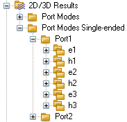
	In case that broadband port modes are calculated (usage of broadband waveguide ports or full deembedding feature), the broadband info of the modes is listed in a special folder (see port info view or port mode view for more details).
	If adaptive mesh refinement is activated in the solver parameter settings the corresponding results can be accessed from this entry, see Adaptive Meshing (Transient), Adaptive Meshing (Eigenmode), Adaptive Meshing (Frequency Domain).
	The results of an evaluation of a field along a curve can be accessed from this entry.

S-Parameter views

Depending on the solver that was used to calculate S-Parameters, there are two types of view possible: the complex view and the classical view. In the classical view you may choose the visualization type by selecting the corresponding tree item named after the visualization type. In the complex view, you may select the tree item and then choose the visualization type from the plot toolbar.

Classical view		Complex View

	The magnitude of the S-parameters is plotted in a linear as well as in a logarithmic scale and also the phase is available.		The S-Parameters will be plotted in the view mode that is set in the plot toolbar: By default, the dB-scaled magnitude of the S-Parameters is shown. Possible views that can be selected are the real part, the imaginary part, the magnitude, the dB-scaled magnitude, the phase and the polar coordinates of the S-parameter. If impedances are available, the S-Parameters can also be plotted in a Smith Chart.
	The S-Parameters are plotted in polar coordinates.
	The S-Parameters are plotted in a Smith Chart.
	If some ports are stimulated simultaneously the magnitude and phase of the signal spectrum at the ports are given as F-Parameters. These values are normalized to the spectrum of the input reference signal. Please note that F-Parameters also show the outgoing results at ports in case of plane wave excitation. More information about F-Parameters and active S-Parameters in case of simultaneous excitation is given on the Reference Value and Normalizing page.		For a description of the F-Parameters, please refer to the classical view. In the complex view, F-Parameters can be visualized exactly like S-Parameters as described above.
	All relevant signals concerning the S-Parameters calculated from the AR-Filter, assuming that it has been activated. To start the AR-Filter, choose Results AR-Filter....		For a description of the AR-Filter results, please refer to the classical view. In the complex view, AR-Filter results can be visualized exactly like S-Parameters as described above.
	The S-Parameters based on the AR-Filter results are plotted in polar coordinates.
	The S-Parameters based on the AR-Filter results are plotted in a Smith Chart.

	The Voltage Standing Wave Ratio can be calculated from the scattering parameters by choosing Post Processing: Signal Post Processing S-Parameter Calculations Calculate VSWR
	The scattering parameters can be converted into impedance and admittance parameters by choosing Post Processing: Signal Post Processing S-Parameter Calculations Calculate Z and Y Matrices
	The Sensitivity Analysis can be currently calculated via the frequency domain solver. For every design parameter a folder with the derivative of the linear magnitude and the phase of the scattering parameters is written.
	The scattering parameter sensitivity can be converted into impedance and admittance parameter sensitivity by choosing Post Processing: Signal Post Processing S-Parameter Calculations Calculate Z and Y Matrices
	The Yield Analysis can be calculated after a successful Sensitivity Analysis computation via Post Processing: Signal Post Processing Yield Analysis. The nominal, lower and upper bound of the linear magnitude and phase of the scattering parameters are plotted.

Simulation control views


	The time dependence of the field energy is plotted.
	The energy balance of the S-Parameters is plotted. This value is only of interest if no open boundary is selected.
	The energy balance of the S-Parameters based on the AR-Filter results is plotted. This value is only of interest if no open boundary is selected.
	In the power folder spectral results of various power curves are plotted.

Creating user defined tree items

It is possible to define user-defined result folders. To do so, select the 1D Result Folder and open the context menu. You will find the following:

New Tree Folder: Creates a user defined subfolder in the selected 1D result folder

Copy: Copies a 1D result curve to the clipboard. You may also press CTRL+C after having selected the desired curve.

Paste: Pastes a previously copied result into a user defined folder. You may also press CTRL+V to paste the previously copied curve into the chosen user defined folder. Also CTRL+V pastes the copied data into various other programs such as Microsoft EXCEL or any ASCII editor.

When selecting a user defined folder some more actions are available:

Scale Result Curve(s): Scale curve(s) enables to scale the x and y axis.

Import Result Curve From ASCII file: Use Import Curve From ASCII file to add two column ASCII data to the project.

CST微波工作室培训课程套装，专家讲解，视频教学，帮助您快速学习掌握CST设计应用

上一篇：CST2013: Farfield Overview
下一篇：CST2013: Port Mode View

CST培训课程推荐详情>>

最全面、最专业的CST微波工作室视频培训课程，可以帮助您从零开始，全面系统学习CST的设计应用【More..】