CST2013: Excitation Functions

Simulation: Sources and LoadsSignalNew Excitation SignalSignal type

In the Excitation Signal dialog, you may select from the following excitation functions. Some of these functions are only available for low frequency or CST MPHYSICS STUDIO solvers.

Overview

Common time functions

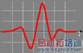
Gaussian

The stimulation is performed with a Gaussian pulse. To define a Gaussian-shaped excitation function a frequency range (Fmin, Fmax) must be specified.

This signal type is relevant in particular for high frequency calculations and is used there as default excitation function.

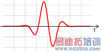
Gaussian sine

This excitation function is similar  to the Gaussian pulse. However, it does not contain any DC part in its spectrum if Fmin is greater than zero.

If results at relatively low frequency are of interest choose the default Gaussian over this excitation function.

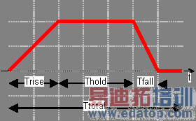
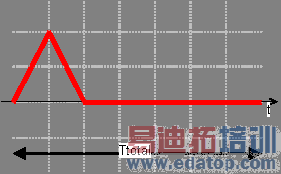
Rectangular

Enables you to define a digital excitation. Use Ttotal, Trise, Thold and Tfall to define the shape of the function. A step function can be obtained by setting Trise and Tfall to zero.

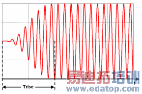
Sine step

Enables you to define a sine step excitation. The parameters Frequency and Phase specify the parameters of the modulation with the sine function. The maximum Amplitude is reached after t=Trise.

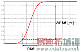
Smooth step

Enables you to define a smooth step excitation, whose amplitude grows from 0 (start) to 1 (end) amplitude. The parameters Trise and Arise [%] specify the slope of the signal, in term of its rise time and the amplitude (in per cent notation) rise interval. In the following picture, for instance, Arise=80%, denoting a growth interval between 10% - 90% value. The definition of the rise interval is always assumed symmetric with respect to 50% value. In a similar way a rise interval between 20% - 80% value is specified by Arise = 60%.

Double exponential

Enables you to define a double exponential excitation using the following expression.

f (t) = A (exp (-t / B) - exp (-t / C))

A: Amplitude

B: Tfall

C: Trise

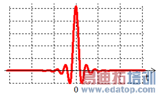
Impulse

Enables you to define an impulse excitation.

A highest required output frequency (Fmax) should be specified to define the shape of this signal.

This signal is centred about zero. It starts at t = -6.25 / Fmax and ends at 6.25 / Fmax. Outside this range, the signal is zero.

User defined

The edit button opens the VBA editor that lets you define an excitation function. Please note that the total time of a user defined signal is always interpreted in the unit seconds.

Example:

 Option Explicit

 Function ExcitationFunction(dtime As Double) As Double

  If ( dtime < 1.0e-9) Then

   ExcitationFunction = 1.0e9 * dtime

 ElseIf ( dtime < 2.0e-9 ) Then

  ExcitationFunction = -1.0e9 * dtime + 2

Else

   ExcitationFunction = 0

 End If

 End Function

Import

Enables you to import a two-column table from an ASCII file which contains the time and signal data. Please note that the data of an imported signal is always interpreted in the unit seconds.

Low frequency time functions

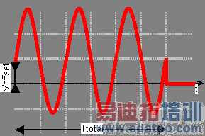
Sine

Enables you to define a sine-shaped excitation. The parameters Voffset and Frequency specify the vertical offset of the sine function and the number of periods within one second (depending on the predefined frequency unit setting), respectively. After Ttotal time units the signal will fall to zero.

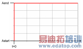
Heavyside step

Enables you to define a Heavyside step excitation. The parameters Astart and Aend specify the amplitude values before and after t=0. At t=0 the function value is Astart.

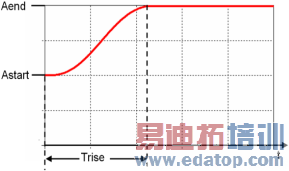
Polynomial step

Enables you to define a polynomial step excitation. The parameters Astart and Aend specify the start and end amplitudes. The end amplitude is reached after t=Trise.

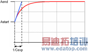
Exponential step

Enables you to define a exponential step excitation. The parameters Astart and Aend specify the start and end amplitudes. Cexp is the exponential constant which determines the functions gradient. At t=0 the gradient is: Cexp*(Aend-Astart)..

Constant

Yields the same constant value 1.0 for all time steps. This signal is used as default in low frequency calculations. It has no meaning for high frequency calculations.

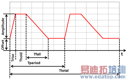
Trapezoidal

The trapezoidal signal is a periodic function with an offset and a trapezoidal pulse whose amplitude is scaleable.

The definition is very similar to the one of the rectangular signal except that the offset and the amplitude is available in addition.