CST2013: Network Parameter Extraction Overview

The network parameter extraction is used to derive a SPICE-compatible network model. Two different methods are implemented to obtain the SPICE network from previous results of solver runs. The first method is based on a transmission line model with a fixed topology of network elements, the second one is based on model order reduction (MOR), enabling an arbitrary topology of network elements.

Overview

Network parameter extraction based on transmission line models

The transmission-line based network parameter extraction is used to derive a SPICE-compatible network model consisting of lumped R, L, C, G, K elements from previously calculated S-parameters.

The transmission-line based network parameter extraction is best suited for a network of coupled transmission lines as it occurs in connectors, IC packages, stripline networks, etc. Based on a fixed topology of the model, the lumped element parameters are adjusted such that the lumped element network response matches closely with the response of the distributed system.

The following sections explain the topology of the model and how the network parameters are calculated from the S-parameters that are assumed to be previously calculated. The parameter extraction currently supports S-parameters calculated with the transient solver or the frequency domain solver.

A single transmission line

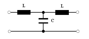
In a first step, let us consider a simple loss-free transmission line (here a microstrip line) that can be modeled quite accurately by a T-shaped network model if the transmission line is electrically short (less than a tenth of a wavelength).

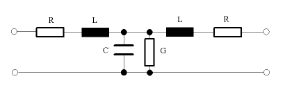
For lossy structures, a serial resistance may be added to the inductance and a parallel resistance may be added to the capacitance. The resulting model is then:

If the transmission line is electrically longer than approximately one tenth of a wavelength, it is important that the lumped network model can also describe the wave propagation along the lines. In such cases, a cascaded transmission line network can be used, where the number of cascades may be specified. A large number of cascades increases the complexity of the model but also improves the accuracy of the approximation. As a general guideline, one cascade for each tenth part of a wavelength should be used. Thus, if the transmission line length is about one wavelength, ten cascades should be used to obtain sufficient accuracy.

The following picture shows the cascaded transmission line model:

A coupled network of transmission lines

Thus far, only a single transmission line has been considered. In the next step, the investigation is extended to a network of two parallel transmission lines (here microstrip lines) as shown in the following picture:

The crosstalk between coupled transmission lines can be described with coupling capacitances (C) and coupled ideal transformers (K). The following picture shows the topology of a coupled network of two transmission lines:

Summary

The topology of the network model is determined by the number of coupled transmission lines and the number of cascades.

The parameters of the lumped elements are calculated from the S-parameters of the three dimensional structure analysis such that the response of the lumped element model matches closely with the given response of the physical device. Therefore, an extraction frequency is specified to set the upper frequency limit for which the approximation needs to be accurate. The upper frequency limit should be set as high as needed, but not much higher than necessary because the error level for the approximation increases with the bandwidth.

Network parameter extraction by model order reduction (MOR)

The network parameter extraction by model order reduction is based on already-calculated S-parameters of previous solver runs. These results are used to determine a significant subset of system poles allowing to remodel the S-parameters with a SPICE compatible network. This network consists of resistors, capacitors, inductances and controlled sources. In contrast to the transmission line based network parameter extraction, the topology of the resulting SPICE model is not fixed.

For the practical usage of this extraction technique, it is required to calculate the full generalized S-matrix of the structure first.

MOR Example

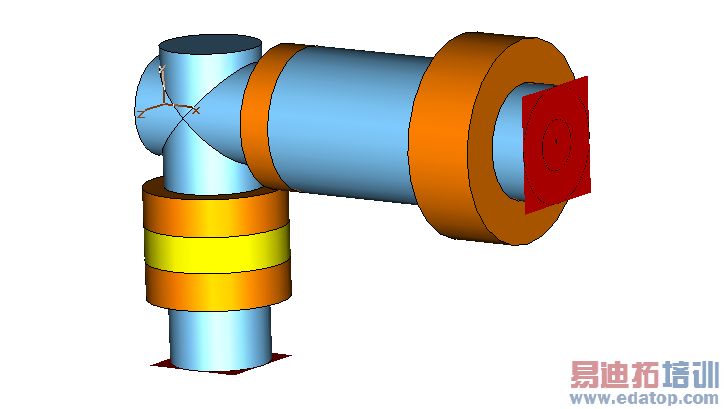
Let us now consider an example and derive an equivalent SPICE circuit for the coaxial connector.

Once all generalized S-parameters have been calculated (All Ports option, no re-normalization to a fixed port impedance), open the dialog box by choosing Post Processing: Signal Post Processing Network Parameters Model Order Reduction...:

In most cases, you can accept the default settings and click the Start button. If you need an HSPICE netlist you can switch the Netlist format checkbox to HSPICE. Then the netlist is generated with a set of Laplace blocks which can be read by Synopsis' HSPICE.

After the network parameter extraction calculation is complete, you should carefully check its output in the message window:

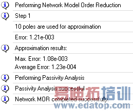
First, check whether the network extraction has completed successfully or whether any warning or error messages have been issued. The generated Berkeley SPICE netlist file containing a subcircuit representing the actual S-parameter data will then look as follows:

******************************************************************

*** Netlist for Macromodel generated by CST DESIGN ENVIRONMENT ***

*** This file was generated automatically                      ***

*** Berkeley SPICE format                                      ***

******************************************************************

*** Generated  07-Aug-2007, 15:32                              ***

******************************************************************

*** Connect the external circuit to ports 1, 2 ..... ***

.subckt Model 1 2

*** Nodal Ckts Associated With Each State Variable ***

Cn1    node1  0    1e-9

Ra1_1   node1  0    3.087219429310181e-002

Ga1_3   node1  0  node3  0   -6.555237103062142e+001

Gb1_1   node1  0  1  0   -2.000000000000000e+000

** End of Nodal Ckt for State Variable #1 **

Cn2    node2  0    1e-9

Ra2_2   node2  0    3.087219429310181e-002

Ga2_4   node2  0  node4  0   -6.555237103062142e+001

Gb2_2   node2  0  2  0   -2.000000000000000e+000

** End of Nodal Ckt for State Variable #2 **

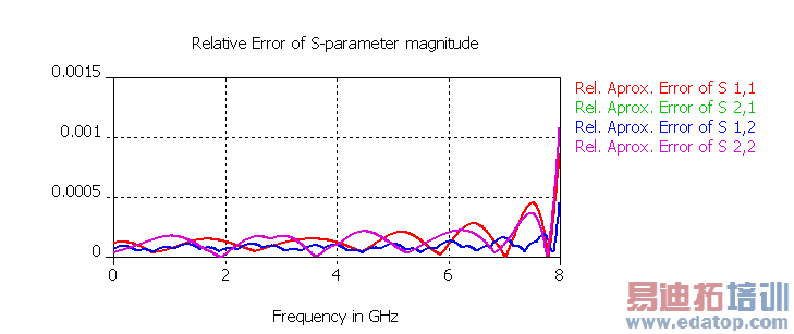
Having verified that the calculation was successful, you should then look at the approximation error which is significantly low for the entire frequency band in this example.

Furthermore, the passivity requirements are met which means that the equivalent SPICE circuit is stable and passive and therefore ideally suited for embedding in larger systems or circuit simulations.

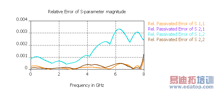
Some more information about the results of the network extraction can be found in the navigation tree’s Navigation Tree 1D Results Network Extraction folder. Check the agreement of the original data and the data provided by the model order reduction by selecting the Navigation Tree 1D Results Network Extraction Error Relative |S| linear folder:

Also the following entries can be found in the navigation tree:

• Approximated S: Shows all S-parameters which have been approximated by a rational function in order to get the system poles for generating the netlist.

• Approx. Error of S: Shows the relative approximation error over the frequency.

• Norm of S: Shows the matrix norm of S for original, approximated and, if enabled, passivated S-parameters over the frequency.

• Passivated S: Shows all S-parameters which have been approximated and passivated.

• Passivated Error of S: The error of the passivated S-parameters over the frequency.

A final verification of the generated netlist can be obtained by loading the netlist into the schematic and comparing its S-parameter results with the original block data.

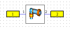
Now switch to the schematic  view by clicking the corresponding tab and add two ports to the CST MICROWAVE STUDIO block representing the current 3D structure. The schematic view should then look as follows:

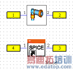
You should now place a SPICE file block into the schematic by dragging it from the block selection tree, Data Import folder. When you are asked to select a netlist file, simply browse for the file which has previously been generated by the SPICE netlist extraction tool. After adding ports to the netlist block again, you should obtain the following schematic:

The impedances of port 1 is 49.46 Ohm and of port 2 is 50.82 Ohm. You have to set these impedances also to port 3 and port 4, respectively. You can do this by double-clicking on port 3 and select Fixed impedance in the General tab and specify the value. Repeat this for port 4.

Running an S-parameter circuit simulation and looking at the results for S1,1 and S3,3 will produce a plot as follows:

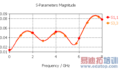
As the picture shows, there is excellent agreement between the results obtained by the circuit simulator using the extracted netlist and the original S-parameter data.

See also

Network Parameter Extraction (Transmission Line) Dialog, Network Parameter Extraction (MOR) Dialog