- 易迪拓培训,专注于微波、射频、天线设计工程师的培养
CST2013: Signals in Time Domain Simulations
录入:edatop.com 点击:
In the following some basic information and functionality regarding time and frequency signals is summarized.
Introduction
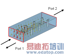
The time domain solver calculates the development of fields through time at discrete locations and at discrete time samples. Every structure must have at least one port where the fields can propagate into or out of the structure. At these ports, voltages and currents are monitored that are the input and output signals of the structure.
Model:
|
T | Time Signals:
|
? |
| ? |
System:
|
T | Scattering Parameters:
|
According to these signals, the transfer functions of the structure are calculated. At this stage, the structure can be considered as an abstract system with input and output signals that are related by the calculated transfer functions, in our case the scattering parameters (S-parameters).
S-Parameter
The S-parameters are defined as the quotient between the output signal spectrum and the input signal spectrum. Therefore the signal spectra have to be calculated. This is done by using the Discrete Fourier Transform (DFT).
Accuracy of the calculated S-Parameter
The S-parameters can only be as accurate as the signals they were calculated from. This means that, theoretically, the S-parameters are only exact if the time signals have entirely come down to zero. Otherwise, information about the system will be lost that would be needed for exact transfer functions.
However, in the simulation, the time signals will never come down. Even when the fields have been propagated entirely through the structure, numerical errors will prevent the signals from reaching zero. At this time, where the signals contain only numerical noise, the simulation should stop because the signals contain no further information about the system. Therefore, a criterion must be found to decide when numerical noise starts to dominate. Also, this criterion should be variable to save simulation time if a lower accuracy is needed.
S-Parameter Balance
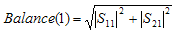
The S-parameter balance is calculated as the square root of the summed power leaving the structure through all ports. The balance should be one for structures that are loss-free (no material losses, no lumped element R) and closed (no open or lossy boundary condition). The power balance indicates frequencies where power is absorbed inside the structure or radiated through open boundaries, e.g., in case of a two port problem the balance regarding excitation at port one is defined as:
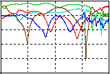
S-Parameter Symmetries
If the modeled structure is symmetric with regard to a set of S-parameters, the number of ports that need to be stimulated may decrease. As a consequence, the calculation time decreases as well. You may save the time for the stimulation of one port if the S-parameters that depend on the stimulation of this port are equivalent to S-parameters that depend on the stimulation of other ports, e.g., if S22 = S11 and S12 = S21, then the stimulation of port 2 is not necessary because S22 and S12 may be copied from S11 and S21.
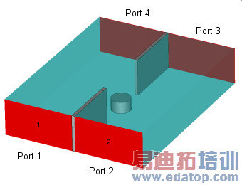
The following picture shows an example for a structure with four ports. Due to the geometric symmetries, S12 = S21 = S34 = S43. However, to reduce the input for the user, it is always assumed that the S-parameter matrix is symmetric, i.e., Spq = Sqp for all ports of the structure. Therefore, you only have to specify the symmetry S21 = S43 (see the dialog box for S-Parameter Symmetries).
Model:
| Symmetry settings:
|
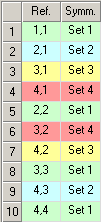
For this structure, only port 1 must be stimulated to obtain all S-parameters. All highlighted S-parameters in the following table can be copied from a S-parameter of stimulation port 1. This reduces the calculation time by a factor of ca. 4.
S11 | S12 = S21 | S13 = S31 | S14 = S41 |
S21 | S22 = S11 | S23 = S32 = S41 | S24 = S42 = S31 |
S31 | S32 = S41 | S33 = S11 | S34 = S43 = S21 |
S41 | S42 = S31 | S43 = S21 | S44 = S11 |
Note: Do not confuse S-parameter symmetries with symmetry planes.
Loss free (Reciprocal) System Detection
Structures with loss-free, isotropic materials have symmetrical transfer functions. This means that in the example of a two-port system, the scattering parameter S21 is equal to that of S12. In this case, only one simulation must be performed to obtain the entire scattering matrix.
The energy balance (see above) is used to detect whether the structure should be treated as loss free or not. A limit can be set and if the balance is lower than this value (over the entire frequency range), the structure is assumed to be loss free.
However, if the limit specified in the steady state energy monitor is high, the low accuracy of the energy balance (and with it the scattering parameters) may cause the detection to fail. Then, it might detect a lossy structure although the structure is, in fact, not lossy.
The appropriate Input Signal
By default, a Gaussian pulse is used as input signal for the time domain simulation. This is ideal, especially for the S-parameter calculation. Its transformed frequency domain signal is also of Gaussian shape and its main advantages are:
A limited bandwidth: this ensures that a mesh can be created where all stimulated frequencies can be properly sampled.
No zero axis crossings: this allows calculation of the S-Parameter over the frequency band of the Gaussian pulse. If there were zeros in the signal spectrum, the S-Parameters could not be calculated at these frequencies.
The choice of the bandwidth to be simulated may have a strong influence on the simulation time. From signal theory, it is known that a narrow bandwidth is related to a quite long time signal. For the field updating scheme, the maximum usable time step is fixed such that a longer input signal requires more simulation time than a shorter signal. Therefore, the best input signal is one that covers the entire frequency range up to the maximum frequency of interest. Do not increase the frequency beyond what you are interested in because this would lead to more mesh points and a smaller time step. Also, for waveguides, you should (if possible) try to choose the frequency above the cut-off frequency of the modes of interest because around cut off there are very slow-traveling waves that again take a long time to simulate.
Besides the Gaussian shaped input signal, it is also possible to define rectangular as well as user defined signals or import a text file containing a data list description. Please refer to the Excitation Signal Dialog for further explanations.
Even if several different time signals can be defined, only one represents the reference signal and is used in general for excitation of a transient simulation. This reference signal can be changed using the context menu and is marked in red and green in the Navigation Tree as described on the Excitation Signal View page.
Steady State Monitor
The criteria that decides when to stop the simulation used in the CST MICROWAVE STUDIO depends on the total energy remaining inside of the calculation volume. If the total energy decreases below a definable limit, the simulation automatically stops. Also, a maximum simulation time can be set to stop the simulation at a defined time.
Another criterion for when to stop the simulation is calculated by the AR-Filter (see below).
Signal Windowing
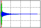
When the simulation has been interrupted such that the signals still have significant values, the cut signal can be thought of as a multiplication of the complete signal by a rectangular time window.
Time Signals: |
|
|
|
|
|
= |
|
* |
|
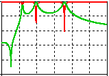
In frequency domain, a multiplication becomes a convolution and a rectangular function becomes a [sin(x) / x] function, where x depends on the window length. With increasing window length, the main maximum narrows, the side maxima of this function decrease, and the zero axis crossings move towards the main maximum. The effect of such a window on the resulting frequency domain signal is that it gets some ripples and its steepness is decreased. However, the locations of the minima and maxima will not change although they might not be visible because of the low steepness of the curve.
Therefore, the rectangular window can be replaced by a squared cosine shaped window. Such a ”filter” lowers the ripples, but again lowers the steepness of the resulting signal.
For highly resonant structures, use the AR-filter to obtain a smoother curve. An AR-filter of good accuracy will not falsify the shape of the scattering parameters (see below).
AR-Filter
The ”Auto Regressive Filter” may be used to shorten simulation time for highly resonant, loss-free structures (or structures with negligible losses). These structures have in common that they need a long time until the energy has propagated out of the resonant parts of the structure and that the signals are ”very periodic” after the main resonating modes have been established inside of the structure. This is the point the AR-Filter attempts to utilize. It tries to predict the relatively simple shape of the signals. However, the predicted signals itself may not have a physical meaning. Only if the energy balance of the signals has acceptable values then the scattering parameters obtained from the AR-Filter can be regarded as valid (see also AR-Filter Overview).
Simultaneous Port Excitation
To calculate S-parameters, the port modes must be stimulated sequentially. However, electromagnetic field distributions may be calculated anyway with multiple port modes stimulated simultaneously. Instead of S-parameters, normalized spectra can be calculated in this case with the Digital Fourier Transform (DFT). Even if each port might be excited with a different time signal, the normalization refers to the previous selected reference signal. As described on the Excitation Signal View page the reference signal can be changed via context menu and is indicated by a red and green icon in the Navigation Tree.
The stimulation signal of the port modes may differ from one port to another. For each port mode, it is possible to specify the magnitude of the signal and a time shift to vary the stimulation start among all the port modes.
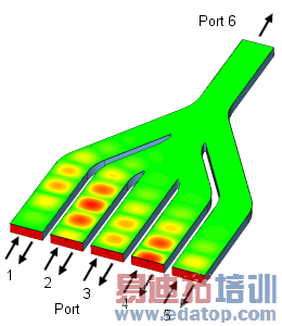
The following picture shows a structure with six ports, where five port modes are stimulated simultaneously at the ports 1 to 5. There is a constant time shift between the port modes. Thus, the stimulation starts first at port 1 and last at port 5. In addition, the magnitude of the stimulation signal at the ports 2 and 4 is twice as high as at the ports 1, 3 and 5.
Model:
|
T
T
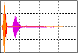
| Time Signals:
? Normalized DFT magnitude:
|
Note: Due to the superposition of the signals and due to the magnitude of the signals, the normalized DFT magnitude may be greater than 0.
TDR Analysis
CST MICROWAVE STUDIO allows the online analysis of the impedance profile along a TEM or similar structure based on the reflected time signals at a port (mode). TDR computation (Time Domain Reflection) is well known from measurement, where TDR is the only possibility to ”look into a structure” and locate mismatches. Typically TDR is applied to TEM structures such as connectors or IC packages designed to have minimum return loss. CST MICROWAVE STUDIO with its transient solver is ideally suited for this task, since TDR pulses have to be short in time (to be able to resolve discontinuities in space) and thus extremely broadband.
The TDR profile can be calculated with two kind of excitations: 1) step time signal or 2) Gaussian time signal. The solver automatically recognizes the signal type and switches between the different TDR calculation methods 1) and 2):
1) Step time signal
A rising rectangular pulse as excitation signal is the typical pulse for TDR evaluation. It has however the disadvantage, that the energy is not decaying (time signal never stops) as well as that the frequency data such as S-Parameters has some "undefined frequencies" due to zero-amplitudes in the excitation spectrum. Both disadvantages do not appear when exciting with a Gaussian pulse. That's why using a Gaussian pulse according to method 2) is recommended.
”Z(t)” is the TDR impedance, ”Z0 ”is the port line impedance, ” i” is the amplitude of the input step signal. ”o(t)” is the reflection signal.
Note: In order to resolve the stimulated highest frequencies in time and space by the discretization, you should choose the upper frequency limit to at least 1/Trise.
2) Gaussian time signal
When using a Gaussian pulse, the TDR is calculated from the time integral of the pulse, which again is the well-known (smooth) step function.
”Z(t)” is the TDR impedance, ”Z0 ”is the port line impedance, ” i(t)” is input Gaussian signal . ”o(t)” is the reflection signal.
Note: The rise time in this case correlates to the upper limit of the frequency band. The frequency range should be adjusted to fmin=0, fmax=”0.876 / rise time”. The rise time is the 10% to 90% rising time of a corresponding step signal, which is the result of an integrated Gaussian pulse.
Example: if the rise time should be 35 ps, then fmax = 0.876/35ps = 25.14GHz. You can see the Gaussian pulse below. The integral of this pulse gives you the step signal with 35ps 10% to 90% rise time.
|
|
Calculate Reflection Factor
With use of the VBA command Solver.TDRReflection "True" the solver calculates the reflection factor over time instead of the time domain reflectometry (TDR). The reflection factor is bound between -1 and +1. Therefore even for an open transmission line, the reflection factor stays within these limits - in contrast to the TDR, which is infinite in this case. The reflection factor is also useful, if the structure needs to be optimized, hence the reflection minimized.
CST微波工作室培训课程套装,专家讲解,视频教学,帮助您快速学习掌握CST设计应用
上一篇:CST2013: Voltage Monitor Mode
下一篇:CST2013: Which Solver To Use
CST培训课程推荐详情>>
 最全面、最专业的CST微波工作室视频培训课程,可以帮助您从零开始,全面系统学习CST的设计应用【More..】
频道总排行
- CST2013: Mesh Problem Handling
- CST2013: Field Source Overview
- CST2013: Discrete Port Overview
- CST2013: Sources and Boundary C
- CST2013: Multipin Port Overview
- CST2013: Farfield Overview
- CST2013: Waveguide Port
- CST2013: Frequency Domain Solver
- CST2013: Import ODB++ Files
- CST2013: Settings for Floquet B