CST2013: Which Solver To Use

CST MICROWAVE STUDIO currently offers different kinds of solver modules. The availability of these solvers depends on your license file (see License Management).

Time Domain Solver

Two time domain solvers are available, both based on hexahedral meshes. These solvers are remarkably efficient for most high frequency applications such as connectors, transmission lines, filters, antennas etc. and can obtain the entire broadband frequency behavior of the simulated device from a single calculation run.

Transient solver: The Transient solver is based on the Finite Integration Technique (FIT). In combination with the Perfect Boundary Approximation (PBA)? feature and the Thin Sheet Technique™ (TST) extension this solver is able to  increase the accuracy of the simulation substantially in comparison to simulation techniques which employ a conventional hexahedral mesh.

TLM solver: The TLM solver uses the Transmission Line Matrix (TLM) method to provide you with accurate broadband results and offers a very efficient octree-based meshing algorithm which efficiently reduces the overall cell count. This solver is especially well suited to EMC/EMI/E3 applications.

In the Time Domain Solver Parameters dialog box you can select the Transient or the TLM solver by choosing the Hexahedral or Hehahedral TLM mesh type, respectively. Please see Time Domain Solver Overview for more details on the general properties and differences of these two solver types.

Frequency Domain Solver

Like the transient solver, the main task for the frequency domain solver module is to calculate S-parameters. Due to the fact that each frequency sample requires a new simulation run, the relationship between calculation time and frequency steps is linear unless special methods are applied to accelerate subsequent frequency domain solver runs. Therefore, the frequency domain solver usually is fastest when only a small number of frequency samples need to be calculated. Hence, a broadband S-parameter simulation with adaptively chosen frequency samples is performed to minimize the number of solver runs. Especially for lower frequency problems with a small number of mesh cells (e.g. 50,000) the frequency domain solver may be an interesting alternative to the transient solver. If a direct equation system solver can be applied for the given problem, which depends on the amount of memory available, the simulation time does not increase significantly with the number of ports and modes. Furthermore, the frequency domain solver may also be useful for strongly resonant structures because these are marked by long settling times of the time domain signals (see Frequency Domain Solver Overview). In addition, electric and magnetic field monitors can be calculated in a postprocessing step very quickly at a given frequency marker (see Calculate field at axis marker in the 1D-Plot Overview).

An alternative method in the frequency domain is the "Resonant: Fast S-Parameter" solver, which calculates S-parameters and fields in the case of a tetrahedral mesh and S-parameters in the case of a hexahedral mesh. For this method, one simulation run is performed to obtain the S-parameters for the entire desired frequency range (see Frequency Domain Solver Overview - Resonant: Fast S-Parameter).

If field monitors are required in the case of a hexahedral mesh, the the "Resonant: S-Parameter, fields" solver can be used. The S-parameters are again calculated in one simulation run for the entire desired frequency range (see Frequency Domain Solver Overview - Resonant: S-Parameter, fields). In addition, electric and magnetic field monitors can be calculated in a postprocessing step very quickly at a given frequency marker (see Calculate field at axis marker in the 1D-Plot Overview).

Eigenmode Solver

In cases of strongly resonant loss-free structures, where the fields (the modes) are to be calculated, the eigenmode solver is very efficient. This kind of analysis is often useful for determining the poles of a highly resonant filter structure. But of course there are different applications for the eigenmode solver: with periodic boundaries and a non-zero phase shift for instance, the eigenmodes are traveling waves. The eigenmode solver directly calculates the first N frequencies for which fields may exist in the structure, and the corresponding field patterns. In case of the JDM eigenmode solver and the eigenmode solver with tetrahedral mesh a frequency target could be chosen such that the eigenmodes are calculated from the frequency target in ascending order. The eigenmode solver can not be used with open boundaries or discrete ports. Electrically lossy materials can be handled by the lossy JDM eigenmode solver method if the assumption of a complex frequency independent permittivity is valid. Alternatively, material losses e.g. for Q-Calculation can be introduced by a perturbation method as a post processing step (see Eigenmode Solver Overview).

Integral Equation Solver

The areas of application for  the integral equation solver are S-Parameter and Farfield/ RCS calculations. The integral equation solver is of special interest for electrically large models. The discretization of the calculation area is reduced to the object boundaries and thus leads to a linear equation system with less unknowns than volume methods.  The system matrix is dense. For calculation efficiency the equation system is solved by the Multi Level Fast Multipole Method (MLFMM). The integral equation solver is available for plane wave excitation and discrete face ports. Electric and open boundaries are supported. Far field monitors and surface current monitors can be set in the Frequency Domain Solver with surface mesh. A broadband S-parameter simulation with adaptively chosen frequency samples is performed to minimize the number of solver runs. For electrically small problems a direct solver is available. The integral equation solver may also be useful for any other open problem (see Integral Equation Solver Overview).

MultilayerSolver

The multilayer Solver is a 3D planar electromagnetic solver for planar modeling and analysis. It is based on the Method of Moments (MoM) and enables users to simulate multilayer geometries accurately and efficiently. The solver features an automatic layer stack generation from a 3D model, automatic edge mesh refinement as well as an automatic de-embedding of ports. Typical applications are RF designs such as planar antennas and filters as well as MMIC and planar feeding network designs. Accurate co-simulation together with CST DESIGN STUDIO for complex micro-strips and transmission lines in 2D becomes with the new multilayer solver easier than before, and together with CST's new System Assembly and Modeling (SAM) you can use the new solver to simulate planar components of complex systems now more efficiently. (see Multilayer Solver Overview).

Asymptotic Solver

The asymptotic solver complements the integral equation solver for very high frequencies. The solver is based on a ray tracing method (shooting and bouncing rays, SBR) which becomes very efficient for monostatic and bistatic scattering and imaging calculations for electrically very large objects. The calculation can either be done by scattering independent rays (more robust for geometrically complex structures) or by using ray tubes (faster for electrically very large objects). The solver currently supports only RCS and farfield calculations for PEC scattering objects together with open boundaries and vacuum background materials (see Asymptotic Solver Overview).

Thermal Stationary Solver

The thermal stationary solver can be used to simulate temperature distribution problems.

For detailed information please refer to the Thermal Stationary Solver Overview page.

Thermal Transient Solver

The thermal transient solver can be used to simulate time-dependent temperature distribution problems.

For detailed information please refer to the Thermal Solver Overview page.

Structural Mechanical Solver

The structural mechanical solver can be used to compute structural deformations resulting from EM-, thermal- or mechanical induced stress. For detailed information please refer to the Mechanical Solver Overview page.

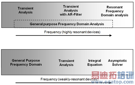
The following figure shows the areas of optimal operation for the different solvers:

General Hints

Please consider the following general hints on how to increase the performance of your simulation runs.

• Always make use of geometric symmetry planes and of all known S-parameter symmetries.

• Avoid an unnecessarily large calculation domain size.

• Consider splitting the structure into smaller parts and combining them in CST DESIGN STUDIO.

• Consider using the multi-processor or distributed computing options.

See also

Mesh and Simulation, Transient Solver, Frequency Domain Solver, Integral Equation Solver, Asymptotic Solver, Eigenmode Solver, Thermal Stationary Solver Structural Mechanical Solver