- 易迪拓培训,专注于微波、射频、天线设计工程师的培养
CST2013: 1D Plot Overview
This page provides an overview of the different 1D plot features. Every one-dimensional result plot may be configured in numerous ways to ease the results analysis.
A plot window will open once a 1D result is selected in the navigation tree. Additional plot windows can be created by selecting 1D Plot: New Plot Window. The plot properties of each window can be set separately. Anyway, all frequency or time dependent plots share a corresponding x-axis. The plot type is dependent on which item is selected in the tree.
When a tree item is selected, the plot toolbar shows possible visualizations of the result. Depending on the result type, only some of the following toolbar icons may be active:
| shows the real part of the result |
| shows the imaginary part of the result |
| shows the magnitude of the result |
| shows the dB-scaled magnitude of the result |
| shows the phase of the result |
| shows the result in polar coordinates |
| shows an impedance Smith Chart of the result |
| shows an admittance Smith Chart of the result |
Cartesian Plot
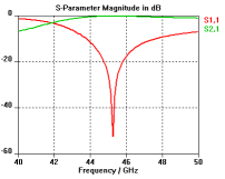
In an cartesian plot the 1D values are plotted in a cartesian system where the abscissa holds the function parameter and the ordinate holds the function value. The plot is labeled according to the signals it contains. The labels of the graphs can be found on the right side of the plot and they are of the same color and style as the graph they belong to. |
|
Polar Plot
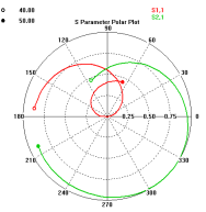
In a polar plot, complex values can be represented. The abscissa holds the real parts and the ordinate holds the imaginary parts. In this plot, both the real and the imaginary values are functions of the independent parameter. Therefore, the parameter itself cannot be read explicitly. In polar plots, the distance from the origin to the graph is the absolute value and the angle from the real axis is the phase of the complex variable. |
|
Smith Chart
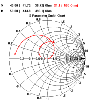
The smith chart is very similar to the polar plot. It also plots complex values where the real and imaginary parts are functions of the independent parameter. The difference is that the axes are transformed from the ”reflection parameter space” into the ”impedance space.” That is, straight lines become circles and circles become straight lines. Smith Charts are defined only for reflection parameters (S11, S22 etc). Therefore, only these values are plotted. |
|
Impedance Norm: The transformation from reflection coefficient to impedance values is made according to
 .
.
This definition assumes a constant normalizing impedance . For this impedance, the line impedance is usually used.
However, for some structures (like wave guides with TE/TM modes) there is no reasonable definition for a line impedance. In these cases a Smith Chart is plotted anyway. The curve label will be modified to point out that the reference impedance is variable. It is clear that in this case the circles (and arcs) in the Smith Chart are not lines of constant real (or imaginary) part of the impedance. Nevertheless it's possible to access the corresponding complex impedance value of every reflection coefficient by placing a curve marker (explained below) on the curve.
If the scattering parameters are re-normalized by hand to an arbitrary value, the user-defined impedance will be taken as the normalizing impedance for the Smith Chart.
General Plot Features
The following general plot features are available:
Zoom and Pan
Holding down the left mouse button and dragging will zoom into the view.
Holding down the middle mouse button and dragging will pan the view.
Pressing space or selecting Reset View from the context menu will reset the view.
The current plot mode can be changed by selecting Zoom Mode or Pan Mode from the 1D plot context menu, which will define the view operation that is performed when holding down the left mouse button and dragging.
The zoom state of a tree item is remembered until the view is reset. Selecting a different item in the navigation tree will not destroy the zoom state of the currently selected tree item.
Curve Markers
Curve markers will display the current ordinate and abscissa value in an additional legend window. If 1D Plot: Curve Markers  Add Curve Marker or Add Curve Marker in the context menu of an arbitrary 1D plot window is selected, the plot mode (zoom or pan) will be temporarily disabled. Now a curve marker can be set on a desired point of a result curve by a left double click on the corresponding location. After the double click the previous plot mode will be switched on again. This feature can also be accessed by pressing 'm' on the keyboard.
Double clicking on a curve marker will open an additional dialog. Here the marker can be moved to a specific value or it can be deleted. This dialog also allows setting multiple curve markers at the specified value to all the result curves of the current plot. It is possible to remove all curve markers of a plot by selecting 1D Plot: Curve Markers  Remove All Curve Markers. It is also possible to remove a single curve marker by hovering the mouse cursor over the marker and pressing the 'delete' key on the keyboard.
Annotations
Annotations can be added to any desired result plot by selecting 1D Plot: Annotations or Add Annotation... in the context menu of the plot window. Annotations will be stored separately for every 1D plot.
Select Curves
Selecting a subset of the currently shown curves can be done using the Curve Selection Dialog.
Curve Style
The line style, line thickness and colors of the plotted curves can be changed using the Curve Style Dialog.
Plot Properties
The plot ranges of the plotted curves can be changed using the Plot Properties Dialog which can be found under 1D Plot Properties for cartesian plots and under Smith Chart and Polar Plot Properties for Smith Chart and Polar plots.
Cartesian Plot Features
The following special plot features are available for cartesian plots:
Axis markers
It is possible to enable an axis marker in any cartesian plot by selecting 1D Plot: Axis Marker or Show Axis Marker in the context menu of the plot window. All frequency (or time) dependent plots like S-Parameters and Balance share the same axis marker object. The axis marker has a legend that shows all values of intersection of the marker and the curves in the plot. Different features are available for the axis marker:
Axis Marker... : will open an additional dialog in which the axis marker can be moved to a specified abscissa value. This feature can also be accessed by pressing the 'tab' key or by double clicking on the axis marker.
Move Axis Marker to Minimum: moves the Axis Marker to the abscissa coordinate with the smallest ordinate. If some curves are highlighted by double clicking on the curves (or the corresponding legend labels), the marker will move to the minimum of the highlighted curves.
Move Axis Marker to Maximum: moves the Axis Marker to the abscissa coordinate with the largest ordinate. If some curves are highlighted by double clicking on the curves (or the corresponding legend labels), the marker will move to the maximum of the highlighted curves.
The following features can be accessed once an axis marker is enabled:
Bond Axis Marker Window: If the legend window of the axis marker was dragged to arbitrary location of the plot window this feature will attach it to the marker again. Double clicking on the axis marker legend window in the plot has the same effect.
Calculate fields at axis marker: This selection will be enabled if an axis marker is shown and if a frequency domain solver has been used that is able to calculate fields. Choosing this option calculates additional electric and magnetic field monitors at the frequency of the current axis marker position. The calculated results are added to the "2D/3D Results" entry of the navigation tree.
Measure Lines
It is possible to enable measure lines in any cartesian plot by selecting 1D Plot: Measure Lines or Show Measure Lines in the context menu of the plot window. All frequency (or time) dependent plots like S-Parameters and Balance share the same measure lines object. It's possible to drag the measure lines to arbitrary locations in the plot domain which makes it easy to measure distances in the direction of the ordinate or the abscissa. Double clicking on one of the measure lines opens a dialog which allows specifying the value of the measure line.
 最全面、最专业的CST微波工作室视频培训课程,可以帮助您从零开始,全面系统学习CST的设计应用【More..】
频道总排行
- CST2013: Mesh Problem Handling
- CST2013: Field Source Overview
- CST2013: Discrete Port Overview
- CST2013: Sources and Boundary C
- CST2013: Multipin Port Overview
- CST2013: Farfield Overview
- CST2013: Waveguide Port
- CST2013: Frequency Domain Solver
- CST2013: Import ODB++ Files
- CST2013: Settings for Floquet B


