- 易迪拓培训,专注于微波、射频、天线设计工程师的培养
CST2013: Discrete Port
录入:edatop.com 点击:
 Simulation: Sources and Loads
  Discrete Port
Besides waveguide ports or plane waves, the discrete ports offers another possibility to feed the calculation domain with power. Three different types of discrete ports are available, considering the excitation as a voltage or current source or as an impedance element that also absorb some power and enables S-parameter calculation.
|
|
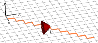
The discrete port is defined by a start point and an endpoint. These two points will be connected by a perfectly conducting wire (visualized by a thick orange line) and the respective port source (indicated by a red cone) in the center of this wire. The colors of the wire and the cone can be changed in the Colors View Options dialog. | Note: The wire between the start point and endpoint of the discrete element must be located along mesh edges. However, in the Modeler View (left picture), the definition of the discrete port will be shown, which is a straight line connecting the two points. Only in the Mesh View (right picture), the actual fitting of the wire to the mesh will be shown. |

A discrete port can also be attached to an end of an existing thin wire. It is only allowed to add one port at an end of a thin wire. The settings for attaching a discrete port to a thin wire can be done in the location frame of this dialog.
Properties frame
Port type: Select here the type of the discrete port. The input parameters in the properties frame will change to correspond with this setting. Please note that the input signal for the port is normalized differently, depending on the chosen port type.
S-Parameter: This port type is modeled by a lumped element, consisting of a current source with inner impedance that excites and absorbs power. The current source will only be active when the discrete element is the stimulation port in the transient analysis.
The current is injected only into the mesh cell where the central part of the port is located (represented by a red conical shape, see pictures above). This lumped source element is perfectly electrically connected along mesh edges with the end points of the defined discrete port (represented by the orange line in the upper right picture) . Along the wire the current behaves like along a transmission line, that means at a particular time the current amplitude can vary along the line.
If a very accurate model of the electrical connection is required (e.g. for an exact bondwire representation), it is recommended to keep the port wire length well below the wavelength of interest and to model the electrical connection by using realistic solids.
This discrete port type realizes an input power of 1 W and enables the calculation of the corresponding S-parameter, based on the incoming and outgoing time signals. In addition, it is possible to monitor the voltage across and the current through the discrete port. Note that the orientation of the discrete port is used to determine the phase of the S-parameters. An equivalent circuit diagram for a discrete port of the S-parameter type is shown below.

Voltage: This port type realizes a voltage source, exciting with constant voltage amplitude. If this port is not stimulated in the transient analysis, the voltage along the wire is set to zero. The voltage excitation signal will be recorded during the solver run.
Current: This port type realizes a current source, exciting with constant current amplitude. The current excitation signal will be recorded during the solver run.
Name: Select a valid name from the drop-down list. This number will be displayed next to the discrete port in structure plots and will be used for naming the S-parameter results. Please note that the port numbers are shared with the waveguide port definitions.
Label: Here, you may define a label for the port.
Impedance / Voltage / Current: Specify a numerical expression for the input parameter of the discrete port. Insert either impedance, voltage amplitude or current amplitude due to the settings made in the port type frame. For the S-parameter selection, the resulting S-parameters will be automatically normed to the specified impedance.
Radius: Define a radius for the port. The port still is represented infinitely thin in the mesh.
Monitor voltage and current: If this option is activated, the voltage across and the current through the discrete port are monitored during the simulation. The resulting time and frequency domain curves are placed in the navigation tree folder 1D Results Discrete Ports Voltages and 1D Results Discrete Ports Currents, respectively.
Please note that the spectral amplitude results represent peak values and are normalized to the spectrum of the defined reference signal. In case of the S-parameter discrete port type, all results refer to an input power of 1 W.
Location frame
Type: Choose 'Coordinates' if the discrete port should be defined by start- and endpoint. Or choose 'Wire' if the discrete port should be attached to an existing thin wire.
X1 / Y1 / Z1: Specify numerical expressions for the global coordinates of the discrete port’s start point. The automatic mesh generation will try to set a mesh node at this position.
X2 / Y2 / Z2: Specify numerical expressions for the global coordinates of the discrete port’s end point. The automatic mesh generation will try to set a mesh node at this position.
U1 / V1 / W1: Specify numerical expressions for the local coordinates of the discrete port’s start point. The automatic mesh generation will try to set a mesh node at this position.
U2 / V2 / W2: Specify numerical expressions for the local coordinates of the discrete port’s end point. The automatic mesh generation will try to set a mesh node at this position.
Use pick: When this option is activated, the start or end points of the discrete port will be taken from the last or second-to-last picked point.
Invert Direction: Exchanges the start point and the endpoint of the discrete port.
Position: Defines the end of the wire, on which the discrete port is attached to. Possible values are 'end1' or 'end2'.
OK
Stores the current settings and leaves the dialog box.
Preview
Press this button to create a preview of the port. This option is very useful to check the settings before you actually create the port.
Cancel
Closes this dialog box without performing any further action.
Help
Shows this help text.
Discrete Port Overview, Waveguide Port, Discrete Face Port, Reference Value and Normalization, Frequency Domain Solver Overview - Resonant: Fast S-Parameter, Frequency Domain Solver Overview - Resonant: S-Parameter, fields
CST微波工作室培训课程套装,专家讲解,视频教学,帮助您快速学习掌握CST设计应用
上一篇:CST2013: Farfield Source
下一篇:CST2013: Define Displacement Boundary
CST培训课程推荐详情>>
 最全面、最专业的CST微波工作室视频培训课程,可以帮助您从零开始,全面系统学习CST的设计应用【More..】
频道总排行
- CST2013: Mesh Problem Handling
- CST2013: Field Source Overview
- CST2013: Discrete Port Overview
- CST2013: Sources and Boundary C
- CST2013: Multipin Port Overview
- CST2013: Farfield Overview
- CST2013: Waveguide Port
- CST2013: Frequency Domain Solver
- CST2013: Import ODB++ Files
- CST2013: Settings for Floquet B