- 易迪拓培训,专注于微波、射频、天线设计工程师的培养
HFSS15: Selecting a Far-Field Quantity to Plot
录入:edatop.com 点击:
When plotting far-field quantities, the quantity can be a value that was calculated by HFSS such as antenna gain, a value from a calculated expression, or an intrinsic (inherent) variable value such as frequency or theta.
To select a far-field quantity to plot:
1. When you create the report, specify the Report Type as "Far Fields."
2. In the Report dialog box, select one of the following Categories for the field setup:
Variables | Intrinsic variables, such as frequency or theta, or user-defined project variables, such as the length of a quarter-wave transformer. |
Output Variables | User defined expressions applied to derive quantities from the original field solution. |
rE | The selected component of the radiated electric field, which is multiplied by the radial distance, r. |
Gain | Gain is four pi times the ratio of an antenna’s radiation intensity in a given direction to the total power accepted by the antenna. |
Directivity | Directivity of the antenna. |
Realized Gain | Realized gain is four pi times the ratio of an antenna’s radiation intensity in a given direction to the total power incident upon the antenna port(s). |
Axial Ratio | Axial ratio of the electric field. |
Polarization Ratio | Polarization ratio of the electric field. |
Antenna Params | HFSS-calculated quantities that include peak directivity, radiated power, accepted power, radiation efficiency including the total and component values at Phi and Theta, max U, and array factors. For far-field setups, the decay factor for lossy materials is calculated as a constant for all far fields. |
Normalized Bistatic RCS | For designs with plane incident waves. RCS is not supported for other types of incident waves. The normalized radar cross section.
where l0 is the wavelength of free space. |
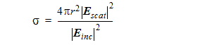
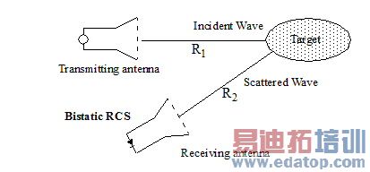
Radar Cross-Section (Bistatic RCS) | For designs with Plane Incident Waves. (RCS is not supported for other types of incident waves). The radar cross-section (RCS) or echo area, s, is measured in meters squared and represented for a bistatic arrangement (that is, when the transmitter and receiver are in different locations as shown in the linked figure). This is represented by
where • Escat • Einc |
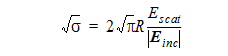
Complex (Bistatic) RCS | For designs with Plane Incident Waves. (RCS is not supported for other types of incident waves) The equation for complex (bistatic) RCS is calculated as:
where • Escat • Einc This form retains the phase information. |
Monostatic RCS | For designs with Plane Incident waves. (RCS is not supported for other types of incident waves) A proper incident angle sweep should exist at the incident wave source setup before HFSS can plot Monostatic RCS. The radar cross-section (RCS) or echo area when the transmitter and receiver are at the same location. For Monostatic RCS, you need not be concerned with the Theta and Phi values defined in the radiation sphere. Only the incident wave Theta and incident wave Phi are used in calculating a Monostatic RCS plot. |

Each Category item that you select causes the Quantity list to offer quantities appropriate to selected category. Category selection for a Variable of an Output Variable lists those available in each case. Selecting Antenna Parameters as Category causes the Quantity list to show Antenna parameters.
3. Select the Quantity to apply to the selected Category.
If the Category item you select is rE, Gain, Directivity, or Realized Gain, you will need to specify the polarization of the electric field by selecting from the Quantity list. This ability to plot the gain of certain vector components (polarizations) of the electric field allows you to evaluate how well your antenna radiates in desired polarizations.
Total | The combined magnitude of the electric field components. |
Phi | The phi component. |
Theta | The theta component. |
X | The x-component. |
Y | The y-component. |
Z | The z-component. |
LHCP | The dominant component for a left-hand, circularly polarized field. |
RHCP | The dominant component for a right-hand, circularly polarized field. |
CircularLHCP | The polarization ratio for a predominantly left-hand, circularly polarized antenna. |
CircularRHCP | The polarization ratio for a predominantly right-hand, circularly polarized antenna. |
SphericalPhi | The polarization ratio for a predominantly f-polarized antenna. |
SphericalTheta | The polarization ratio for a predominantly q-polarized antenna. |
L3X | The dominant component for an x-polarized aperture using Ludwig’s third definition of cross polarization. |
L3Y | The dominant component for a y-polarized aperture using Ludwig’s third definition of cross polarization. |
The plot’s Y axis field shows the combined selections.
For example, if you select Gain as the Category, and RHCP as the Quantity, HFSS evaluates the equation as follows:


4. You can also select a function to apply to the your selections for the Category and Quantity (for example, mag).
As you make selections in the Report dialog for Category, Quantity, and Function, the Y field shows the combined calculation they describe.
5. Click New Report to create the Report.
The new report based on your selections is displayed.
HFSS 学习培训课程套装,专家讲解,视频教学,帮助您全面系统地学习掌握HFSS
上一篇:Scan Specification for Regular Uniform Arrays
下一篇:Script Method Argument