HFSS15: Defining Frequency-Dependent Material Properties

HFSS provides several frequency-dependent material models. The Piecewise Linear and Frequency Dependent Data Points models apply to both the electric and magnetic properties of the material. However, they do not guarantee that the material satisfies causality conditions, and so they should only be used for frequency-domain applications.

The Debye and Djordjevic-Sarkar models apply only to the electrical properties of dielectric materials. These models satisfy the Kramers-Kronig conditions for causality, and so are preferred for applications (such as TDR or Full-Wave Spice) where time-domain results are needed. The HFSS Design Settings also include an automatic Djordjevic-Sarkar model to ensure causal solutions when solving frequency sweeps for simple constant material properties.

In HFSS, you can assign conductivity either directly as bulk conductivity, or as a loss tangent. This provides flexibility, but you should only provide the loss once. The solver uses the loss values just as they are entered.

1. With respect to a material selected in the Select Definition window, in the View/Edit Material window, click Set Frequency Dependency.

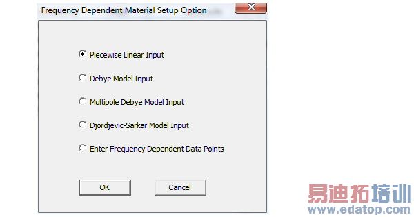
2. In the Frequency Dependent Material Setup Option window, do one of the following:

• Select Piecewise Linear Input. This defines the material property values as a restricted form of piecewise linear model with exactly 3 segments (flat, linear, flat). You will specify the property's values at an upper and lower corner frequency. Between these corner frequencies, HFSS linearly interpolates the material properties; above and below the corner frequencies, HFSS extrapolates the property values as constants. This dataset can be modified with additional points if desired.

• Select Debye Model Input. This is a single-pole model for the frequency response of a lossy dielectric material. In some materials, up to about a 10-GHz limit, ion and dipole polarization dominate and a single pole Debye model is adequate. HFSS allows you to specify an upper and lower measurement frequency, and the loss tangent and relative permittivity values at these frequencies. You may optionally enter the permittivity at optical frequency, the DC conductivity, and a constant relative permeability.

• Select Multipole Debye Model Input. This lets you provide the data of relative permittivity and loss tangent versus frequency. Based on this data the software dynamically generates frequency dependent expressions for relative permittivity and loss tangent through the Multipole Debye Model. The input dialog plots these expressions together with your input data through the linear interpolations.

• The generated expressions provide the new value for the material properties of relative permittivity and loss tangent.

• Both the expressions and data triples can be saved and reloaded.

• Select Djordjevic-Sarkar Model Input. This model was developed for low-loss dielectric materials (particularly FR-4) commonly used in printed circuit boards and packages. In effect, it uses an infinite distribution of poles to model the frequency response, and in particular the nearly constant loss tangent, of these materials. HFSS allows you to enter the relative permittivity and loss tangent at a single measurement frequency. You may optionally enter the relative permittivity and conductivity at DC.

If you try to enter invalid values for the Djordjevic-Sarkar model, you receive error messages.

• Select Enter Frequency Dependent Data Points. This allows you to enter, import or edit frequency dependent data sets for each material property. Any number of data points may be entered. This is an arbitrary piecewise linear model. A simple data set will not provide a causal material.

3. Click OK.

A dialog appears, based on your selection.

Piecewise Linear Input

Debye Model Input

Multipole Debye Model Input

Djordjevic-Sarkar

Enter Frequency Dependent Data Points

After you have entered the data for your selection, you return to the View/Edit Material window. New default function names appear in the material property text boxes. HFSS automatically created a dataset for each material property. Based on a varying property’s dataset, HFSS can interpolate the property’s values at the desired frequencies during solution generation.

To modify the dataset with additional points, see Modifying Datasets.