HFSS15: Surface Roughness Modeling

Surface roughness plays an important role in accurately modeling radio frequency components (RFC), e.g. resonators, and signal integrity projects, like microstrips and printed circuit boards (PCBs). The increase of the surface resistance due to surface roughness results in lower quality factor (Q) in resonators and higher insertion losses for microstrips and PCBs. The scale of the roughness is different in the different application areas so different surface roughness models are used. The common theme in the different models is that an effective frequency dependent conductivity is defined depending on the type and magnitude of the roughness, which shows the increase of the surface resistance compared to the smooth surface resistance.

For RFC projects, Groiss [6] or Hammerstand [4] model may be employed. Groiss model uses an experimental formula:

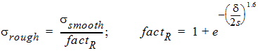
(13)

where s is the surface roughness and d is the skin depth. It can be seen that the maximal ratio is two, so this model is just applicable to RFC problems, where the surfaces are highly polished to avoid lower Q. A surface roughness model of higher losses is necessary to model the fabrication effects in PCBs where the roughness of the deposited metal is considerably higher. The recently developed Huray surface roughness model ([2], [4]) copes with the problem by applying a multiplicative factor:

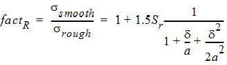
(14)

where S_r is the ratio of the surfaces of all "spheres" found in a cut and the cut surface. a is the radius of the spheres and d is the skin depth. All SIBCs depend on the conductivity explicitly and implicitly as well. The effective conductivity is applied to the explicit conductivity, as (Eqs. (4) - (9)):

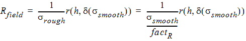
(15)

which similarly applies to the imaginary part of the SIBC. It can be seen that the effective conductivity, s_rough, is frequency dependent, which if not handled correctly can cause causality violations.

There are two ways of avoiding causality violations. One way is to construct a complex impedance factor which satisfies the Kramers - Kronig relations [2]. The other way is to use the known, causal Drude metal model. Drude model is very similar to the Debye model:

(16)

where s_inf and s_smooth are the high frequency and low frequency limits of the conductivity, respectively.t is the reciprocal of omega where the conductivity is about

.

Every surface roughness model behaves the same way: sigma is constant at low and high frequencies; it just changes in a transition region. Knowing s_inf , s_smooth and t from the surface roughness model, a Drude model can be created. Fig. 2 shows how the Drude model approximates the rough sigma of the Huray model. If the accuracy of the approximation is not satisfactory, a multipole Drude model can also be constructed to exactly match the conductivity of the Huray model (similar to Eq. (12)). The Drude model has been applied to a 7 inches long microstrip line.

Figure 2 Frequency dependent conductivity of Huray model (red), real part of Drude model
and imaginary part of Drude model (blue)

Fig. 3 shows the insertion losses. Green, red and blue curves show the measured, Huray model and Drude model cases, respectively. The results were checked by using a causality checker available in ANSYS Designer. Though, the causality violation of the non-causal Huray model is small (0.0083), using Drude model decreases the violation error by about one order of magnitude (to 0.00062)

.

Figure 3: Insertion loss of a microstrip line. Measured (green), Huray model (red)
and Drude model (blue). Resonance is due to fiberglass weave [9].

Next

Deembedding Parasitic Lumped Port Effects